Blessing Texas Case Study

The availability of a small 3D Southeastern Texas gulf coast survey provided an excellent data set for directly comparing single arrival Kirchhoff migration with the much more computationally intensive full waveform reverse time migration. This study concluded that while there is an almost imperceptible difference between vertical time or depth sections, a high resolution fault analysis indicates that the more accurate method produces much higher resolution results. That this is the case, even when neither the geology nor the velocity model indicates any significant lateral gradients, is a bit surprising.

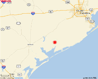
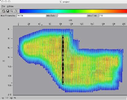
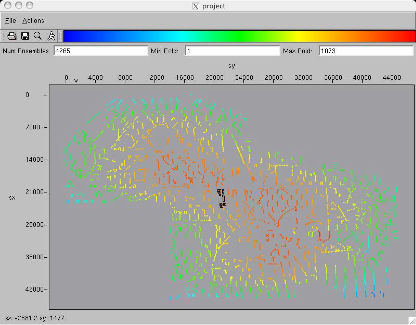
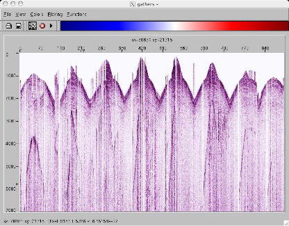
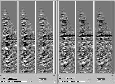
Figure  17 is a graphic montage depicting a 3D seismic survey acquired in the late 1980's or early 1990's near the town of Blessing in the state of Texas in the USA. The graphic in (a) shows the approximate location of the survey, (b) shows the CDP locations and fold, (c) shows the shot locations, and (d) shows an example shot where each shot was acquired by eight lines of receivers. There were approximately 1080 receivers per shot, and there were approximately 4265 shots. There are approximately 4,200,000 total traces in this survey.

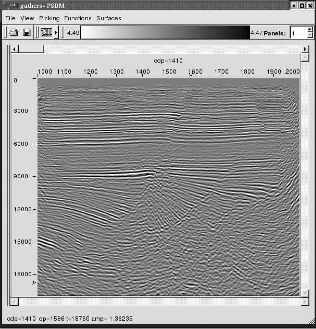
The migration in Figure  18 was one of the first done on the Blessing data. The target is indicated by the yellow square and the question was whether or not this clearly faulted zone contained one or two faults. A secondary question focused on whether the black square does or does not contain a continuation of the fault entering the square at the lower left corner.

Figure 18: A early Kirchhoff prestack depth migration of the Blessing data

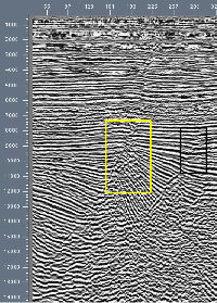
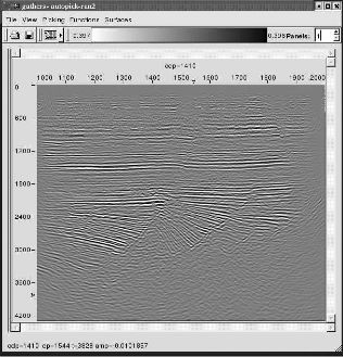
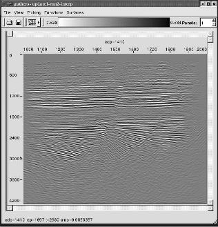
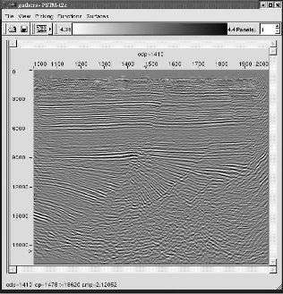
Figure  19(a) shows a straight ray time migration using the first iteration of velocity analysis, while (b) shows the second iteration result. Each of these initial iterations were performed using a semblance-based automatic picking routine. Figure  19(c) shows a curved ray PSTM with the final interval velocity volume. Part (d) is different because it used a migration algorithm that selected a velocity function at the source and another velocity function at the receiver to estimate the required traveltimes.

To ensure the highest possible velocity accuracy, tomography was applied to the Blessing data set. The before and after common image gather comparison in Figure  20 demonstrates that the painless velocity update method was sufficient to ensure high quality imaging.

Figure 20: A before and after comparison of tomography

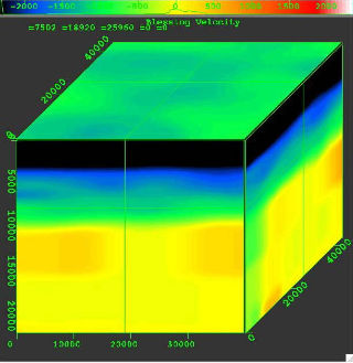
The images in Figure  21 represent the final depth-interval velocity volume and the final Kirchhoff maximum energy depth image at approximately line 1466.

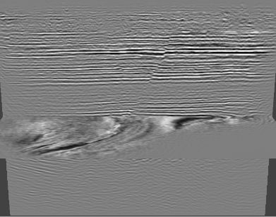
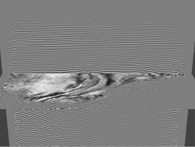
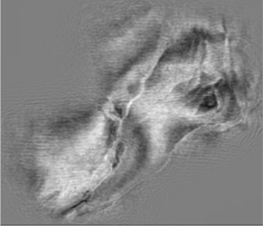
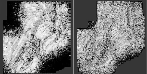
The key points of the images in Figure  22 are that, when viewed in sectional form, there appears to be little difference between the Kirchhoff single arrival in (a) and the much more computationally intensive reverse-time migration in (b). However, when viewed purely as depth slices, as in (c) and (d), the differences between the two methods are clear.

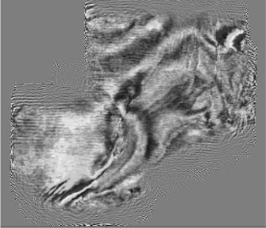
A high resolution fault analysis was run on both the Kirchhoff migration and the two-way volumes to verify the preliminary conclusion that the two-way method is of considerably higher resolution. A visual comparison of Figure  23(a) with Figure  23(b) confirms this basic hypothesis.

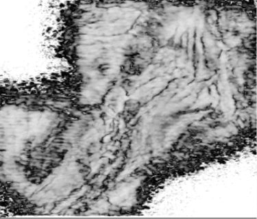
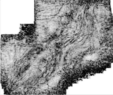
Figure  24 is another high-resolution fault analysis at a slightly different depth. The two-way still shows much higher resolution than the Kirchhoff.

Figure 24: A high resolution fault analysis of a second set of depth slice from the Blessing data volume.