Variational Formulation and Finite Elements

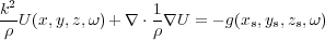
We begin with Equation  18 in the frequency domain, where g ( _s ) is a pressure source located at _s = ( x _s ;y _s ;z _s ), and with = ( x;y;z ), k ( ) = .

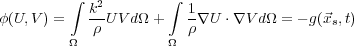
Equation  50 has the variational form in Equation  51, where V is an element of a suitable space V of functions that can be used to approximate U ( ).

(50)

(51)

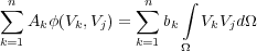
Given a family, V _k, of basis functions spanning V, we can approximate U, and g by U ( ) = P _{k =1} ⁿ A _k V _k ( ) and g ( _s ;! ) = P _{k =1} ⁿ b _k V _k ( ) so that the variational form in equation ( 51) can be expressed in matrix form as Equation  53, where ^T = and ^T = .

(52)

(53)

In this setting, S is called the complex impedance matrix and M is called the stiffness matrix. Note that we have dropped reference to frequency ω so that S = M is a single frequency equation.

If we choose our discretization scheme properly, we may assume that S is square, symmetric, and invertible so that the modeling operator S ¹ generates data according to the formula in Equation  54.

(54)

The key point to this discussion is that we have wide latitude in the choice of the V _k. We can divide the model into a collection of local regions and then define the V _k through polynomials, pyramids, or perhaps even boxes over each of the sub domains. This approach tends to work well when the problem is defined by thing like bridges, aeronautical structures, and other more rigid bodies, but has never gained ground in seismic settings. Mathematically, dividing the medium up in this way is quite difficult, so more modern approaches tend to choose domains that are uniformly square or rectangular. It is also convenient to have basis functions that are easily differentiable and orthogonal Thus, in some sense, the modern version of finite element methods (FEM) tends to look more and more like a very sophisticated finite difference approach. However you accomplish the model division, the need to invert a matrix of significant size remains a serious issue.

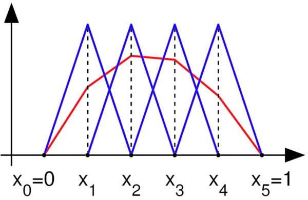
As as an example, consider the one dimensional case and define V _k ( x ) as shown in Equation  55.

(55)

As illustrated in Figure  11, the V _k = 1 ;:::;n basis is composed of shifted and scaled tent functions. For the two-dimensional case, we choose again one basis function V _k per vertex x _k of the triangulation of the planar region . The function V _k is the unique function of x whose value is 1 at x _k and zero at every x _j ; j ≠ k. This process extends easily to three dimensions.

Figure 11: Basis functions V k (blue) and a linear combination of them, which is piecewise linear (red)

The primary advantage of this choice of basis is that the inner product in Equation  56 will be zero for almost all j;k.

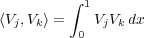(56)

In the one dimensional case, the support of V _k is the interval [ x _{k 1} ;x _{k +1} ]. Hence, the integrands of h V _j ;V _k i and Φ ( V _j ;V _k ) are identically zero whenever j j k j > 1.

Similarly, in the planar case, if x _j and x _k do not share an edge of the triangulation, then the integrals Equation  57 and Equation  58 are both zero.

(57)

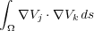(58)

In two-dimensions, triangular elements can be used to approximate the domain of approximation is both regular and irregular ways. In Figure  12, a regular mesh is used to approximate the domain, and then through pyramids approximate the dome-like structure in the figure. Figure  13 shows an much more irregular approximation of the domain of approximation. Figure  12 illustrates a reasonably regular triangular decomposition of a domain at the bottom and the approximation to a dome accomplished through the use of the pyramidal versions of the basis functions in Figure  11.

Figure 12: Domain triangles with pyramids as elements approximate a dome like surface. In this case the triangular basis mesh is regular. ( From Wikipidia)

Figure 13: Domain triangles with pyramids as elements approximate a dome like surface. Here the triangular basis mesh is irregular. ( From Wikipidia)

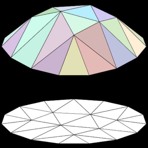
In contrast, Figure  13 is an example of the utilization of irregularly sized triangles to decompose the domain of approximation.

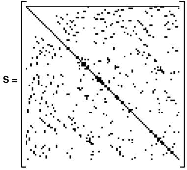
Figure  14 shows the general form of a 2D S matrix. Generally, this matrix has dimensions equal to the number of nodes or finite elements. An intriguing feature of the finite element method is that once the S-matrix is inverted, any and all shot responses can be synthesized from this single inverse.

Figure 14: The general form of the S-matrix in two-dimensions.( From Wikipidia)

Depending on the author, the word "element" in "finite element method" refers either to the triangles in the domain, the piecewise linear basis function, or both. For our purposes, it is the latter. So for instance, an author interested in curved domains might replace the triangles with curved primitives, in which case he might describe his elements as being curvilinear. On the other hand, some authors replace "piecewise linear" by "piecewise quadratic" or even "piecewise polynomial". The author might then say "higher order element" instead of "higher degree polynomial". The finite element method is not restricted to triangles (or tetrahedra in 3D, or higher order simplexes in multidimensional spaces), but can be defined on quadrilateral subdomains (hexahedra, prisms, or pyramids in 3D, and so on). Higher order shapes (curvilinear elements) can be defined with polynomial and even non-polynomial shapes (for example, ellipses or circles).

More advanced implementations (adaptive finite element methods) utilize a method to assess the quality of the results (based on error estimation theory) and modify the mesh during the solution, aiming to achieve an approximate solution within some bounds from the "exact" solution of the continuum problem. Mesh adaptivity may utilize various techniques, the most popular are:

• Moving nodes (r-adaptivity)
• Refining (and unrefining) elements (h-adaptivity)
• Changing order of base functions (p-adaptivity)
• Combinations of the above (hp-adaptivity)

In general, the finite element method is characterized by the following process.

• Choose a grid for Ω. In the preceding example the grid consisted of grid points or nodes, but one can also use triangles or curvilinear polygons.
• Choose basis functions. In our discussion, we used piecewise linear basis functions, but it is also common to use piecewise polynomial basis functions

A separate consideration is the smoothness of the basis functions. For second order elliptic boundary value problems, piecewise polynomial basis functions that are merely continuous will suffice (that is, the derivatives are discontinuous.) For higher order partial differential equations, you must use smoother basis functions. For instance, for a fourth order problem such as u _xxxx + u _yyyy = f, you may use piecewise quadratic basis functions that are both continuous and have first order derivatives.

An Old Movie

We can now use our modeling schema to generate synthetic shot data. Because we have a complete wavefield at each time step, we present the synthetic data in movie form. Our first movie (snapshots in Figure  15) was generated by R. G. Keys (now at ConocoPhillips in Houston, Texas) in February of 1982. At that time, the multiplicity of snapshots comprising these data required about 30 minutes to generate on a Cray 1S supercomputer. Today, almost any modern desktop, and even some laptops, can produce the same movie virtually in real time. As the movie progresses, please note that waves travel in all directions and the wavefield recorded at the top surface of this model would include refractions, reflections, and all forms of multiples.

Figure 15: Snapshot from 1982 Finite Element Pinchout Model synthesis. Figure  15 is a place holder for the actual pinchout movie that will be shown during the presentation.