Raytrace Modeling

Figure  37(a) provides an example of how Huygens principle factors into construction of a raytrace-based response to exploding reflectors. Given a point on a reflecting surface (the red circle in the figure), a ray from a source point simulates an exploding the point. Rays emanate from the point in all directions and are recorded at surface receivers. Since any reflecting surface can be considered as a set of such points, the sum of all their point responses will produce, in the worst case, a reasonable approximation of what we would see if we ran our full two-way propagator for this model.

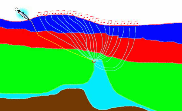
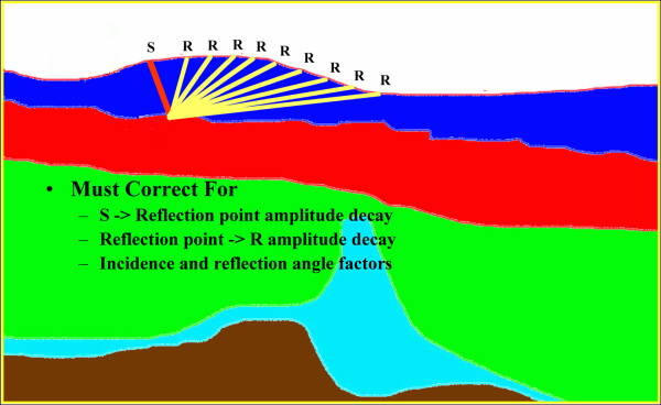
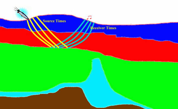
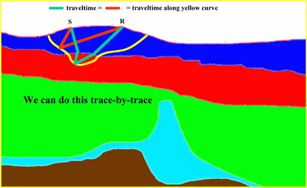
Figure  38 provides proof of concept that the ray-based synthesis methods outlined here actually work. In this figure, the model is on the left and the ray based synthetic shot is on the right. The phase function, φ, and amplitude decays, A, were calculated using the method of characteristics along with a simultaneous solution to the transport equation.

Figure 38: A raytrace shot over the SEG AA' 2D model.

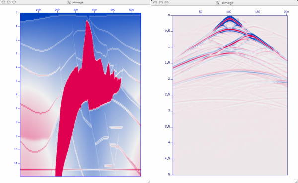
Figure  37(b) hints at one of the more complicated parts of accurate raytrace modeling. Reasonably accurate raytrace amplitude responses require that we correct for several important factors. These include source-to-reflection point decay and reflection-point-to-receiver amplitude decay, as well as obliquity factors based on the incidence and reflection angles. The phase of secondary arrivals also require correction.

Depending on how it is structured, raytrace modeling can be one of the most computationally efficient modeling methods available. It can easily model virtually any type of recording geometry. As indicated in Figure  37(c), raytrace modeling is easily modified to achieve fixed or common offset modeling. Its chief drawback is that multiples and other multiple arrival events are very difficult to include in the modeling exercise.

While we tend to think of raytrace modeling in the sense of the isochron in Figure  37(a), this may not be optimum. Figure  37(d) shows raytrace modeling formulated in terms of equal traveltime curves or surfaces. The yellow curve in this figure represents all the reflection points for which the sum of the traveltime from a source to any point on the yellow line and back to a receiver is identical to that from any other reflection point. To produce the amplitude response at this time requires only that we sum all reflection amplitudes at these locations into the trace at this fixed time. If you already understand Kirchhoff migration to some degree, this concept should be very familiar.

While the raypath concept is, in most cases sufficient, to understand plane wave issues we emphasize that the full plane wave generated by the source is much more complicated. Because of this fact, it is possible to generate a full wave response from an appropriately sampled bundle of ray theoretic plane waves. Figure  39 demonstrates this in terms of what are more precisely called Gaussian Beams. What we see in this figure is part of the full response due to two plane wave raypaths. The blue lines indicate what are called central rays, while the red lines indicate wavefronts calculated directly from the central rays. The wavefronts are actually calculated using a finite difference technique specified by theoretical formulas analogous to those on which our one and two-way propagators are based. In addition to dynamically determining the amplitude at each point on the red lines, a Gaussian weight is applied to ensure that the sum of all such waves faithfully represents the forward traveling wavefront. The name Gaussian Beam is derived from this weighting methodology.

Figure 39: A partial wave response due to two rays.

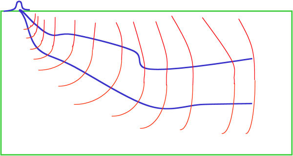
Figure  40 shows the kinds of events that each of our schemes can model successfully.

Figure 40: A brief comparison of modeling methods.

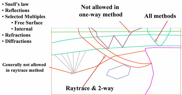
Figure  41 summarizes the differences between three modeling algorithms. The left hand side represents full two-way propagation, the middle image shows one-way propagation, and the right side shows single arrival raytrace based modeling. Note that neither the full one-way nor the single arrival raytrace base response have any reflected waves.

Figure 41: Basic model differences. Left is full two-way, middle is one-way, and right is single arrival Kirchhoff shot response for shot in center of model.