Migration in Time

Time migration moves dipping events from their apparent locations to their true locations in time. The resulting image is shown in terms of traveltime rather than depth, and must then be converted to depth with an accurate velocity model. Because of the clear and direct connection to data synthesis over media described in terms of depth, it is easy to explain depth migration in the time-reversed sense.

However, even though it can be one of the most accurate imaging methods, depth migration has not yet reached the acceptance level it deserves. There are many reasons for this. One reason is the belief by many people that finding the most accurate velocity is still beyond the reach of most depth-migration methods. This was certainly true when actually performing a prestack migration of any form was beyond the reach of the computational capacities of the period. Historically, imaging in time by hand (see Chapter 1) was easy to explain with virtually no need to even consider partial differential equations. Interpreters were required to have only limited mathematical ability to do the migration and could perform all depth conversions as a simple vertical stretch.

Moreover, as shown in Figure  17 and discussed in Chapter 1, interpreters could compute the migration position and time quite easily using only an appropriate RMS velocity and locally estimated dip. Consequently, the coupling of readily available computer power with multi-fold data for estimating stacking velocities led directly to a plethora of time-migration versions of the depth migration algorithms listed in the previous sections.

Converting to Vertical Time

Converting depth migration algorithms into time migration algorithms is not difficult, but the process is not easy to explain fully without detailed mathematical analysis.

In 2D, vertical time, τ, is defined by Equation  13, where z is depth, and v ( x;z ) is a two-dimensional velocity function.

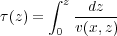(13)

There is, of course, a 3D version of this equation, but for simplicity we will only consider the 2D case.

With this as our variable of choice, the two-dimensional equation governing our wavefield takes the form of Equation  14, which, on the surface, appears to be little different from the depth equation on which all modeling and depth imaging is based.

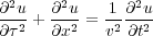(14)

The problem is that this equation has two time variables. One, t, is the actual time governing wavefield propagation, and it is what we record in the form of arrival times. The other, τ, is simply the conversion of vertical depth to time. The key point to all of this is that wavefields do not travel in vertical time, they propagate in space. Therefore, the problem is how can we solve Equation  14 for the image at time τ.

Jon Claerbout (1976) found a unique solution to this problem. He first recognized that vertically propagating solutions of this equation are constant along level lines, t + τ = constant. He then made a change of variables from t to t 0 = t + τ, and then ignored all higher order derivatives. The result is

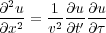(15)

This equation can be solved discretely quite easily. The transformation from Equation  14 to 15 is not unlike the factorization into one-way equations in the Modeling chapter (Chapter 3), and so virtually all of the concepts and ideas incorporated in depth migration algorithms are also part and parcel of the time migration scene. In the same manner that factoring the full two-way equation into two one-way equations theoretically limited propagation to no more than 90 degrees, approximating Equation  14, another easily solvable equation, also reduces the dip response of any image. Perhaps the only significant difference between the one-way depth approach and the one-way time migration approach is that the latter is almost always cast as an implicit scheme. Because the required matrix inversion is relatively simple, this does not result in a computationally intense algorithm. Thus, time migration as practiced in the past is quite efficient.

The Major Difference between Time and Depth Migration

The major difference between time and depth migration is directly related to the transformation from depth, z, to vertical time, τ. This difference is illustrated in Figure  13, which provides a graphic of what happens when the velocity varies in any direction. Depth migration accurately places the imaged event at its image ray time location, while time migration continues to place the migrated event at vertical time. Large lateral placement errors are the rule when the velocity varies strongly. This is a major reason to prefer depth migration over pure time-migration approaches, but it is not the only reason. Ray bending is also extremely limited because time migrations utilize RMS velocities instead of true interval velocities.

Figure 13: The major difference between time and depth.

Dip Limits

As we saw in the chapter on modeling, factoring the full two-way equation limited one-way propagation to 90 degrees, since almost any implementation of a one-way method decreases the dip response. In depth migration, the basic problem arises from the need to approximate the square-root term in the one-way equation. The approximation is usually the result of truncating a Taylor series, but it can also result from other approximations.

In vertical-time migrations, an entirely different equation replaces the fundamental wave equation, but its approximation is the result of truncation and also results in a decreased dip response. This decrease is clearly evident on any comparison between the algorithmic and exact impulse responses. It is not surprising that the recognized definition of dip limits was based on where the impulse response breaks down. Figure  14 shows how dip limits are defined.

Figure 14: Algorithmic dip limit definitions.

Using this definition, it is possible to show that the dip limit of early time migration algorithms did not exceed 15 degrees. Consequently, they were called 15 degree algorithms. Increasing the approximation accuracy by using additional terms in series approximations produced algorithms with 45 and even in some cases 60 degree limits. Using three or more terms ultimately resulted in diminishing returns and there was an upper limit of around 80 degrees. Although there are many different domains of application, the process almost always revolves around some type of series expansion of either the square root term or its time-domain equivalent.

One-Way XT-Time Migration

The simple model shown at the top of Figure  15 was designed to test the basic concepts of zero-offset seismic migration or imaging. The model consists of 16 flat and 16 dipping events in a constant velocity medium, where the first dipping event is actually flat. Since the medium has constant velocity, there is absolutely no difference between running a time or a depth migration algorithm. We will test our first migration by running one-way time migration algorithms that are limited to 15 and 45 degree dip responses. The idea is to see just how good of a job we can do with a more or less naive approach.

Figure 15: Simple constant velocity model with dipping events from 0 to 70 degrees.

The data shown at the bottom of Figure  15 demonstrates several of the usual rules of thumb concerning seismic data. In this case, since the data was synthesized numerically, it is pure zero-offset data; that is, there is no separation between the source and receiver used to synthesize it.

The 15 degree approach shown in Figure  16 exhibits one of the most difficult aspects of migration. Imaging steeply dipping events is very much a function of the accuracy of the approximations used to make the algorithm workable.

Figure 16: Application of a 15 degree equation and the impact of interpolation.

In the lower half of this figure, we see under-migrated events. Visual inspection reveals that the highest correct dip on the section is approximately 20 degrees. This is a bit higher than the 15 degrees the model study suggests is possible, but well within the expected error of the method. The bottom of this figure also demonstrates something called grid dispersion. This phenomenon is a complex part of the algorithm's implementations, but is easily handled by interpolating to a finer sample interval. The top half of the figure demonstrates that although the grid dispersion can be removed quite easily, the improper placement of the steep dips is still apparent.

If we move to a more accurate algorithm, in this case a 45 degree approximation, as shown in Figure  17, we see that we can easily achieve proper placement up to approximately 55 degrees. In this case, grid dispersion is not as much of a problem, even though it is still present. The more accurate implementation has achieved much better overall results.

Figure 17: Application of a 45 degree equation and the impact of interpolation.

One-Way FK Time Migration

One-way FK time migration can be separated into a phase shift migration method and a phase shift plus interpolation (PSPI) method.

Phase Shift Migration

Phase shift migration in time is actually based on an approximation of the transformed wave equation, Equation  15. However, the process of down shifting the surface exploding reflector data is given by Equation  16, where φ is defined by Equation  17. Variable v _rms is the RMS velocity between τ and τ + Δ, and is virtually identical to its depth counterpart given by Equation  123.

(16)

(17)

Phase Shift Plus Interpolation

Phase-shift-plus-interpolation (PSPI) is identical to the process in depth explained in Equation  4. The only noticeable difference is that the down shift takes place in migrated time rather than migrated or imaged depth. Multiple velocities can be phase shifted to form the basis of an interpolation scheme in either space-time or frequency-space to make sure that the process is accurate, effective, and fast.

Kirchhoff Style Time Migration

Kirchhoff style time migration can be separated into straight-ray Kirchhoff time migration and curved-ray Kirchhoff time migration.

Straight-Ray Kirchhoff Time Migration

Straight ray Kirchhoff migration does not really do what the name implies. The method is patterned on Figure  17 and the RMS velocity as defined in Equation  4.

As shown in Figure  18, the method selects an RMS velocity function at the output image location, I, and then uses it in the traditional traveltime Equation  18 to compute the required traveltime from the source to the image point and back to the coincident receiver. Once this time, 2 τ _S, is available, the method selects the amplitude from the trace at surface location S, and adds the output to the location A at time τ.

Figure 18: Straight ray Kirchhoff Migration.

The blue line indicates all image points with the same output migration time. In a constant velocity medium, this equal-traveltime curve is actually a circle and represents the set of points which are equally likely points from which energy might be reflected. This process was the de facto Kirchhoff algorithm for many years and was one of the first to be computerized.

Curved-Ray Kirchhoff Time Migration

Equation  18 is the traditional traveltime formula for the time between a source at a distance from a surface point, m, and an image point located directly below m with a vertical traveltime of τ ₀.

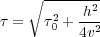(18)

This is a truncation of a series of the form shown in Equation  19, where c ₁ = is the reciprocal of the RMS velocity, v. As shown in Figure  19, the rest of the c _i values are complicated modes of the interval velocity function, v ( iΔz ).

(19)

Figure 19: Curved ray traveltimes.

Figure  20 shows how curved ray Kirchhoff migration works using the full series representation shown in Figure  19.

Figure 20: Curved ray Kirchhoff time migration.

Calculating the traveltime through a velocity medium that varies only in the vertical direction ensures that the migration is identical to those that would be obtained using a raytracer. In effect, a curved ray time migration is identical to performing a depth migration using a different v ( z ) for each output location and then outputting the result in vertical time.

Cascaded Migration

Figure  21 shows how migration algorithms can be cascaded to improve the overall response of the final migration.

Figure 21: Cascaded Migration.

In some cases, the combination of several poor migration techniques produces a migration that is superior to each individual migration methodology. Each successive migration takes place with a migration field that is constructed from a small portion of the final velocity field and a constant velocity. Usually, the piece of the final field is chosen so as not to have any strong variations. After migrating with the constructed field, the next migration begins where the last one left off. That is, the new time zero is defined by the time at which the constant velocity functions intersect that portion of the final velocity field used during this stage of the cascade.

Almost any migration algorithm can be cascaded. The basic problem is that cascaded migrations are theoretically correct only when the cascade is performed after a constant velocity migration. This, in effect, means that the cascade concept can only be applied effectively after a completely straight-ray time migration.