Common Offset Kirchhoff Ray-Based Methods

Kirchhoff migrations have long been a staple of imaging technology. As a result, there are many excellent implementations of this methodology. Almost all are so-called single arrival approaches, whether in time or depth. Generally speaking, when the velocity gradients are reasonable, single arrival methods have excellent capabilities and can produce excellent images. On the other hand, when overburden velocity variations are strong, Kirchhoff methods can have significant problems imaging below these variations.

Straight Ray Kirchhoff Prestack Time Migration

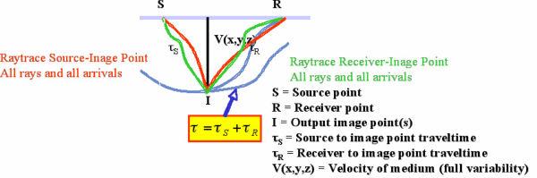
The process described in Figure  20 provides the basic schema for all single arrival prestack Kirchhoff time and depth migrations.

Figure 20: Straight ray prestack Kirchhoff time migration.

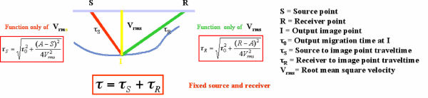
The process gives a simple velocity dependent recipe for computing a source to image-point traveltime and an image-point to receiver traveltime for use in the migration. In this prestack case, a closed form local RMS velocity formula produces the required times. The sum of these two traveltimes is then used to select an amplitude from the trace with this source and receiver. We then calculate a correction amplitude for this image point, multiply it times the amplitude selected from the trace, and add the result to the output image location. To avoid aliasing, it is normal to filter the trace using the usual aliasing equation in Equation  18.

(18)

Equation  18 is used to compute a dip dependent upper frequency to restrict the frequency content of the trace prior to adding the extracted amplitude into the corresponding output image point. The simplest version of this type of anti-aliasing pre-computes several traces with decreasing frequency bands and then selects the desired amplitude from the one most likely to avoid aliasing issues.

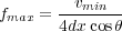
Curved Ray Kirchhoff Prestack Time Migration

The curved ray Kirchhoff prestack time migration algorithm shown in Figure  21 is based solely on the curved ray formulas in Figure  19. Those formulas are used to compute source to image point and image point to receiver traveltimes. Typically, the required v ( z ) velocity is selected at the image point, but it is clearly possible to select one at the source and a different one at the receiver.

Figure 21: Curved-ray-prestack-time-Kirchhoff migration.

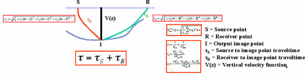
Single Arrival Kirchhoff Depth Migration

As indicated in Figure  22, the only difference between various Kirchhoff prestack time migrations and Kirchhoff depth migrations lies in how the required traveltimes are computed.

Figure 22: Single-arrival-Kirchhoff-depth migraiton

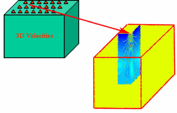
Raytracing is by far the dominant method for calculating these traveltimes. In this figure, rays are traced from the source and the receiver to the output image point. The traveltime sum, along with appropriate amplitude corrections, is then used to sum the trace amplitude into the output image point. On the surface, this process requires that rays be traced from each source and receiver to each output image point. Computing a traveltime volume for each and every source and receiver location can be very expensive, so as shown in Figure  23, most modern Kirchhoff implementations precompute traveltimes on a regular grid.

Figure 23: Raytracing issues for all 3D raytrace based imaging methods

It is possible that more than one ray will arrive at any given image point during the calculation. Since keeping track of every such arrival is an extremely complex bookkeeping problem, it usually easier to choose a single arrival, but the selection of the arrival best serving the migration process is not always easy. Typical arrivals of this type are maximum energy, minimum distance, or minimum velocity.

Minimum velocity arrivals avoid headwaves caused by proximity to salt or other high velocity structures. Thus, in areas with strong lateral velocity variations, such as salt regimes, the minimum velocity methodology is considered to be optimum. In such cases, the minimum velocity ray is defined to be that ray for which the sum of all velocities along the ray has the smallest value. Interpolation is used to compute the desired traveltime at each source, receiver, and image point, thus reducing the overall computation costs and generally improving the speed of the migration step.

Clearly, the accuracy of the migration is controlled by how well the implementation handles both the traveltime computations and the interpolation of the traveltime volumes.

Multiple Arrival Kirchhoff Migration

Energy from a seismic source can reach any given subsurface point in more than one way. Figure  24 characterizes this concept graphically in terms of rays. Each ray is uniquely determined by either its take-off angle or by its arrival (incidence) angle, and there is no restriction on how many rays from a fixed source location can reach any given subsurface point. To properly implement an algorithm of this type we must, at least in theory, calculate an amplitude and a phase-shift for each arrival to correct the selected amplitude from the current input trace.

Figure 24: Multiple-arrival-prestack-Kirchhoff-depth migration

Multi-arrival Kirchhoff migration is very difficult to implement since it presents a rather complex bookkeeping problem that apparently has no efficient solution. This is unfortunate because multi-arrival Kirchhoff migration has the greatest potential for providing an algorithm with a near optimum percentage of the features of full two-way imaging. Based on empirical observations from the myriad implementations of its single-arrival brother, it would have super dip response, excellent amplitude handling, as well as the ability to include turning rays and diffractions.

Kirchhoff Elastic Depth Migration

The separation between acoustic and elastic Kirchhoff migration algorithms is solely determined by traveltime calculations. The migration step is not dependent on how the traveltime volumes are computed. If the traveltime volumes are based on acoustic equations, the result is an acoustic migration. If they are based on anisotropic calculations, the result is an anisotropic migration. If the source traveltimes are based on compressional velocities and the receiver traveltimes are based on shear velocities, the resulting algorithm is a converted wave migration.

Single Arrival Kirchhoff Depth Migration Summary

As the current work-horse of seismic depth migration and migration velocity analysis, single arrival Kirchhoff migration has proven to have excellent dip response, good amplitude response, and has shown some ability to image turning ray energy. Its great flexibility as a velocity analysis tool suggests that it will be around for some time to come. Its single biggest drawback is that it is very sensitive to strong lateral velocity variations, particularly below salt structures. This is very likely due to the use of a single arrival.

Raytrace-based migrations rely heavily on the quality and accuracy of their traveltime generators. As a high-frequency approximation to forward wave-field propagation, raytracing can be very sensitive to even relatively minor velocity variations. Reducing this sensitivity usually means that the input velocity field must be smoothed before calculating traveltime tables. In some cases, this is not an issue, but when the velocity variation is strong, significant depth errors may result. The raytrace module must compute both the traveltime to a given image point and any and all amplitude correction factors. If the raytracer is inaccurate, so is the output image, and no raytracer can recover from an incorrect velocity field. Likewise, no velocity field can be recovered from an incorrect raytracer.

When using Kirchhoff style methods, it is extremely important to understand how, when and where traveltime volumes are computed. If the migration algorithm is based only on downward, single arrival raytracing, then each volume must be sampled sufficiently well in all directions to ensure proper accuracy. In some Kirchhoff implementations, traveltime generators are based on finite difference solutions to the basic Eikonal equation that governs ray propagation. Because Eikonal-based methods are generally only able to calculate first arrivals, they are prone to producing spurious results in complex geological models.

Raytrace methods facilitate the calculation of multiple arrivals, and the selection of the most appropriate arrival better serves the migration process. Raytracing is the preferred traveltime generation method.

The utilization of a single arrival in Kirchhoff depth migration technology is one of the chief reasons these methods have difficulty imaging below complex structures. When we use all of the possible arrivals, as shown in Figure  24, we can achieve a superior result to what is achieved with the single arrival approach. While multiple arrivals complicate the migration algorithm and generally make it more computationally costly, the benefit of including more arrivals usually outweighs the increased cost. However, because it is so difficult to solve the general bookkeeping problem involved in making a multi-arrival Kirchhoff practical, this approach is seldom used.