Zero Offset Modeling
At this point, our understanding of modeling is based on a two-step process. A source of some kind is
initiated at time,
t
= 0, and it is then allowed to propagate into the Earth according to some form of
propagating equation. We also understand that each subsurface point in the Earth, whether part of a
reflector or not, can be considered as a point reflector. After some length of time, energy from the
source reaches the point, and, according to Huygens Principle, initiates a new source at the location
of the point reflector. The point reflector then acts as a internal source which radiates energy in all
directions. Some of this energy reaches the surface as a reflection and some of it continues into the Earth to
ignite other point reflectors creating additional sources until the energy is exhausted. What we record
at the surface is the reflected energy at a widespread array of receivers with some offset from the
source position. What we lose is the energy that never manages to get reflected. In such synthetic
experiments, we can record all the information we want. If desired, we can even record zero-offset
data, but to do that we have to set off sources at each location we want a receiver. This means that at
considerable computational expense, we must forward propagate a source for every coincident receiver
location.
In the early days of reflection seismic processing and interpretation, there was seldom enough computer power to
produce an appropriate number of shots to enable synthesis of stacked sections. It was natural to attempt to find a
way to produce all the traces in zero or short offset ensembles. It does not take much effort to come up with a
reasonable approach. The Huygens principle tells us that if we can determine the response from any single
subsurface point, all we have to do to produce the receiver wavefield is to sum all such responses into the receiver
and we are done. Let's consider the zero-offset response of a single point-reflector. If the traveltime from the
source at
s
i to the point-reflector at,
r, is
t
s
i
r then the traveltime from the reflector back to the source
is also
t
s
i
r. The reason for this is that the energy reaching the receiver at the source position must
travel the path (or paths) from the source to the point-reflector in reverse. This means that the total
traveltime from the source to the reflecting point and back to the receiver at the coincident source location
is just
2
t
s
i. This statement must be true for every coincident source and receiver on the recording
surface, so the zero offset response of the point reflector is the sum of the response for each source,
s
i, on the recording surface. The trick to understanding how to efficiently synthesize a zero-offset
responses is simply to realize that if the velocity,
v, of the medium is divided by two and we set off an
explosion at the point reflector at
t
= 0, then what we will record on the recording surface is exactly the
time
2
t
s
i. Thus, exploiting Huygens Principle in Figure
33, the zero offset response for any given
model can be obtained by simply dividing the velocity by two, setting off explosions at each subsurface
point reflector, and recording the response at the surface. The only problem with this trick is that the
zero-offset response obtained in this fashion will have odd period multiples whenever a free-surface is
present.
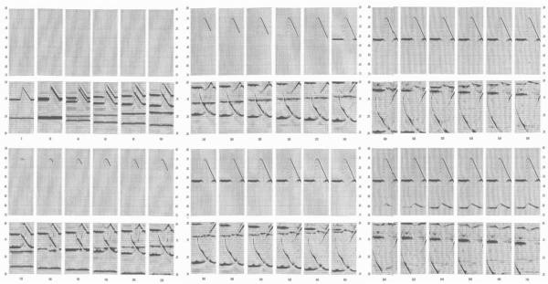
Figure
42 shows us, in detail, what happens in the subsurface, and Figure
43 shows us what we get at the surface
when we synthesize exploding-reflector-zero-offset data.
An easy way to understand the comments in the previous paragraph is through watching the movie schematized in
Figure
44. This move was made in the late 1980's or early 1990's from a model derived from a 3D two-way
migration of
DMO corrected Gulf of Mexico stacked data. It is based on what turned out to be an inaccurate
interpretation of the salt flank, but is still an interesting case study.