Model Boundaries

This section describes the things we must do to handle model boundaries.

Free Surface

Handling a free surface is probably the most complex of the various problems that arise in seismic modeling exercises. The literature on this aspect of the synthesis is quite vast and outside the scope of what we wish to discuss here. We leave detailed investigation of this to you, if you are interested.

However, one of the more appealing methods is discussed by Lavendar in his 1988 paper on P-SV modeling, and illustrated in Figure  25. The essential difference lies in how each layer is handled. Turning on (or off) free surface reverberations controls whether or not synthetic data contains multiples and ghosts.

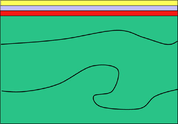
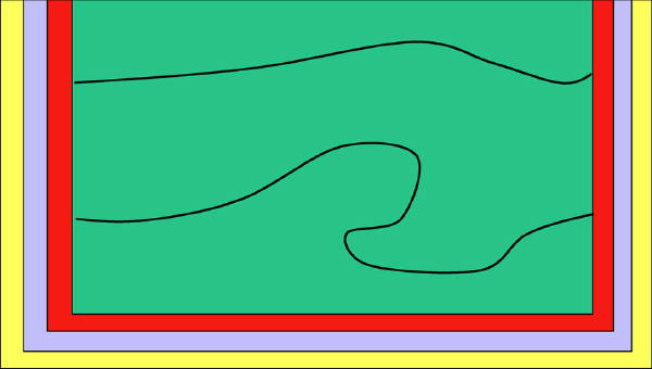
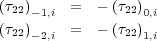
The free surface at the top of the model is padded above with a fictitious set of nodes. Since a free surface implies that no normal or shear stress are active there, we can set τ _{2 ; 2} = 0 and τ _{1 ; 2} = 0 at the top. The shear stress boundary condition is handled by setting it to zero at z = 0 as well. The normal stress is not defined at the top boundary but is forced to zero by making the normal stress antisymmetric for the first two rows above the free surface, as shown in Equation  101.

Non Free Surface

There are a variety of approaches for handling the other boundaries in a typical seismic Earth model. The three most popular are what are called sponge boundary conditions, absorbing, boundary conditions, and the so called perfectly matched layers.

Sponge Boundaries

The idea behind sponge boundary conditions is to modify the propagating equation by adding viscosity to equation along the boundary. This is normally accomplished by writing Equation  102, where 0 γ is an absorbing parameter chosen to produce a wave that decreases in amplitude with distance.

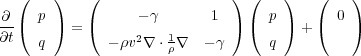(102)

Gamma is usually chosen to have exponential decay within the defined boundary zone and is zero within the model dimensions. Note that when γ = 0, the solution to the equation is, in fact, p.

For the finite element method, sponge boundaries can be implemented by changing the definition of φ ( U;V ) to Equation  103, where α and β are the damping factors in each of the boundary layers.

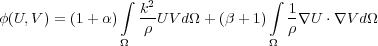(103)

Perfectly Matched Layer

Perfectly matched layers represent a more modern treatment of the sponge boundary conditions. In this setting, the spatial derivatives are modified so that we have Equation  104.

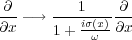(104)

Paraxial Boundaries

Paraxial boundaries are based on the one-way wave equation and within the boundary layers take the form in Equation  105, where j α _j j < for all j (Higdon 1991).

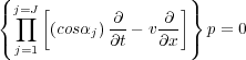(105)

This equation works because each factor cos ( _j ) v is an annihilator of any wave arriving at an angle α _j.

FEM versus FDM Differences

The finite difference method (FDM) is an alternative way of approximating solutions of PDEs. The differences between FEM and FDM are:

• The finite difference method is an approximation to the differential equation while the finite element method is an approximation to its solution.
• The most attractive feature of the FEM is its ability to handle complicated geometries (and boundaries) with relative ease. While FDM in its basic form is restricted to handle rectangular shapes and simple alterations thereof, the handling of geometries in FEM is theoretically straightforward.
• The most attractive feature of finite differences is that it can be very easy to implement and does not require the inversion of an extremely large matrix.
• In some cases, FEM can be considered to be equivalent to an FDM. Choosing basis functions as either piecewise constant functions or Dirac delta functions produce a FDM type method. In both approaches, the approximations are defined on the entire domain, but need not be continuous.
• The FEM is generally considered to be more mathematically sound then the FDM, and more accurate. Typically, the quality of the approximation between grid points is excellent in FEM but poor in FDM.
• The quality of a FEM approximation is often higher than in the corresponding FDM approach, but this is extremely problem dependent. There are numerous examples to the contrary.

Generally, FEM is the method of choice in all types of structural analysis problems, but it has not proven to be of tremendous value in seismic simulation or migration. The biggest reason for this is the tremendous size of the impedance matrix S. This makes handling it quite difficult.

Two-Way Implicit Modeling

With the exception of the finite element method, the two-way approaches described above are what are usually referred to as explicit schemes. They forward march source samples one step at a time. The finite element method is close to what is said to be an implicit approach. Finding the solution requires the inversion of a matrix. There are certainly approaches to seismic modeling that can be framed in an implicit sense, but those are equation dependent and will not be discussed further here.

One-Way Modeling

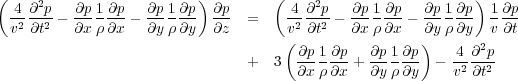
Although its not quite mathematically correct, Equation  17 is sometimes factored into two first order equations. The factorization leads to two separate first-order equations in z which is the product in Equation  106 to illustrate the nature of the factorization.

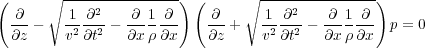(106)

In the case where the density, ρ, is constant, or, even better, equal to 1, the equations simplify further and are what are usually used when applied as part of a migration.

Clearly, the thought process to arrive at this product assumes that the two cross-product terms commute, and thus their difference is zero, but this assumption of commutation is simply not mathematically correct. Nevertheless, is can be shown that suitable approximations to either of the first-order equations that result from the factorization honor the wavefront travel times of the original two-way equation. Because wavefields are no longer allowed to travel in any direction other than upward or downward, the amplitude of the propagation cannot be correct.

In the case of normal full-wave propagation, the impinging wavefield energy creates a new source at the point of impact. Regardless of source wavefield type (that is, compressional or shear), the new source radiates energy in all directions weighted by the reflection strength for upward traveling wave, transmission strength for the downward traveling waves, and angle of the reflecting bed. This is an extremely important concept for all of the discussion that follows. It actually allows us to think in terms of separating wavefields into upward only and downward only propagation directions. Each factor in Equation  106 does precisely that. The first factor governs downward only traveling waves while the second permits only upward traveling waves.

Once a suitable approximation for the term under the square root has been found, almost any of the methods discussed above can be applied to synthesize data of the type specified by the equation. When the downward factor is used, you can propagate wavefields downward but not upward. When the upward factor is used, wavefields can be propagated upward but not downward. Thus, these equations seriously limit the extent to which full wavefield seismic can be generated.

One Way Implicit Finite Difference

There are many known approximations for the square root in Equation  106. Each such approximation has its own pros and cons, and each has its own unique limit to the downward propagation angle it will tolerate. One of the better known square-root approximations is Equation  107.

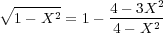(107)

If we apply this approximation to the square root in Equation  106, we obtain Equation  107.

(108)

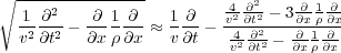
Equation  107 leads directly to a downward propagation equation of the rather complex form in Equation  109.

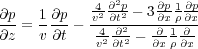(109)

At first glance, this equation may seem to be somewhat intractable for any finite difference approach. The trick to putting this into a more useable form is to clear fractions to obtain Equation  110.

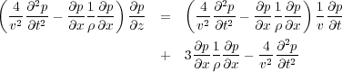
Equation  110 in 3D becomes Equation  111.

If we then approximate the derivatives via some form of the finite difference stencils discussed in previous sections, we can rearrange the problem os solving Equation  109 into a matrix style system of the form in Equation  112.

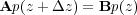(112)

Solving this system amounts to inverting A. The need to employ finite-differences in time can make this a very complicated task in 3D. Consequently this XT method has not enjoyed a lot of popularity in either forward modeling or imaging for 3D projects.