Anisotropic Earth Models

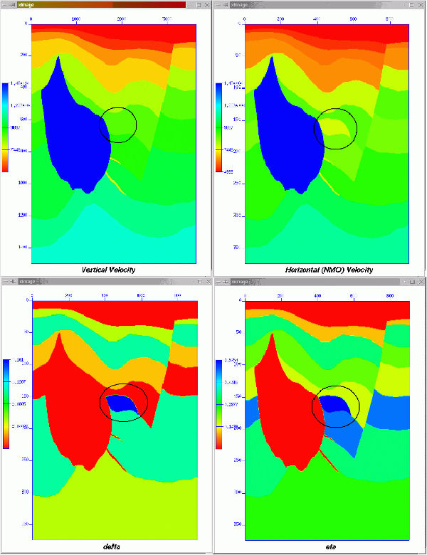
This section provides a simple example of how even simple anisotropic migrations can bring improved imaging to the migration arena. The Earth model in this section is based on an actual exploration problem that arose when drilling revealed a structure that was not apparent in the original imaging exercise. The vertical or well velocity of the highlighted turtle-like structure in the center of the model does not change. It is only the horizontal or NMO velocity that is indicative of its presence.

Figure  15 is an example of a simple 2D anisotropic Earth model. Shown are the vertical or well velocity (top left), the NMO velocity (top right), Thomsen's parameter δ (bottom left), and Thomsen's parameter η (bottom right).

Figure 15: An anisotropic Earth Model.

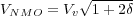
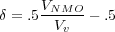
Although this figure contains four graphics, such models can be represented by only three parametric volumes. Given a vertical velocity, V _v, and Thomsen's parameters, δ and ε, we can express any of the others by suitable rearrangement of Equation  1 and Equation  2.

(1)

(2)

From a practical perspective, we usually estimate V _NMO using what has become traditional Kirchhoff based migration velocity analysis.

Since

(3)

it is clear that δ can be estimated through a simple combination of a well velocity and a velocity volume estimated through the usual migration velocity analysis process. Unfortunately, the same cannot be said for ε.

Figure  16 shows a set of images from several experiments to determine the extent to which anisotropic imaging might be of value.

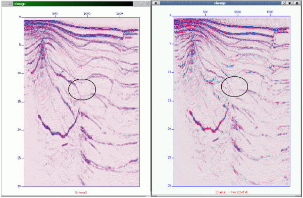
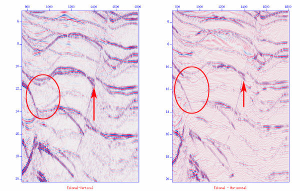
For this purpose, the model in Figure  15 was used to generate a series of shots. Figures 16(a) through (g) are various comparisons using different combinations of the underlying Earth model derived from that in Figure  15. Figure  16(a) and (b) show the results of using either the well velocity or the NMO velocity alone. The turtle back structure in these figures is essentially invisible so there is no reason to suspect its existence. While use of the vertical velocity does produce reasonable depth conversion when the reflecting horizon is relatively flat, steeply dipping events are either not imaged or are misplaced. Use of the NMO velocity tends to get steeply dipping events in their proper place, but does a poor job of depth conversion.

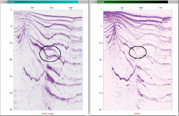
As shown in Figures 16(c) and (d), the issue changes quite quickly when an isotropic shot using the vertical velocity, or a full Kirchhoff anisotropic shot migration is applied. Now, the turtle back structure is clearly visible in both images, and depth conversion is quite good. However, while the shot migration is excellent, several of the steeply dipping events are still misplaced.

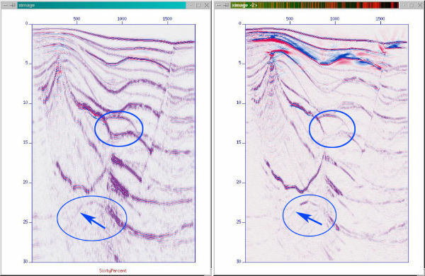
Figure  16(e) compares isotropic shot and Kirchhoff migrations using the vertical velocity. There is no question that the shot migration is worth the effort, but neither of these migrations accurately image steeply dipping events.

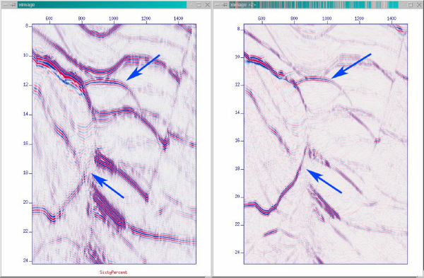
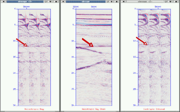
Figure  16(f) shows why anisotropic imaging is worth the effort. The left hand side of (f) shows anisotropically imaged CDP's, while the right hand side shows isotropically imaged CDP's. The middle image is just a representation of the location of the CDP's at the top of the turtle-like structure. The greater flatness, along with improved amplitude response of the anisotropic CDP's, is clear evidence of the need to utilize anisotropic methods when available.