Stacking and DMO

The primary purpose of this section is to provide a simple understanding of why certain parts of early digital processing techniques did not image all of the Earth's structures. This, in effect, is an interpretation issue. We will see that what might be considered easily imaged events are sometimes totally invisible in the seismic record. In many such cases, parts of the subsurface structure may be invisible simply because we have not applied the most accurate available technique to image it. In other cases, its absence may be due to improper noise suppression techniques applied during the preprocessing steps. Whatever the cause, the idea is always to be able to understand what approach produces the best image.

What is Stacking and DMO?

As we will see, migration can be split into four conceptual pieces. As a rule of thumb, these four pieces will help us understand what migration is and how it naturally completes the imaging process.

1.

The first piece is called normal moveout (NMO). When the world is flat, NMO corrects for the fact that the source and receiver are not coincident, but it cannot do so when the reflections come from dipping horizons.

2.

The second piece of migration corrects for dip. Historically, this second piece was called dip-moveout (DMO), but, in the cases of interest here, it happens within the migration methodology itself.

3.

The third migration piece shifts events on each moveout-corrected offset to its true subsurface position.

4.

The fourth and final piece sums (stacks) all the redundant traces into the final image.

When the Earth's velocity has very little lateral variation, these four operations can be split apart and applied in any desired order. The most familiar order is NMO, DMO, stack, and finally migration. However, when the velocity is almost constant, it is quite possible to use the order DMO, migration, NMO, and stack. Full prestack migration can be thought to have the order DMO, NMO, imaging, and stack, but in reality the sequence DMO, NMO, and imaging is usually done in one giant process.

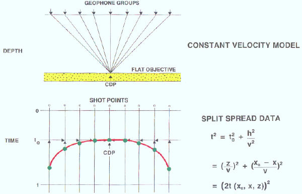
Initial attempts at subsurface imaging forced the geophysicist to join the Flat Earth Society. For a constant velocity medium, Figure  35 shows that Greek mathematics can be used to provide the total travel time, t, from a surface source to a flat subsurface reflector and back to a surface receiver. This is done in terms of the two-way vertical travel time, t ₀, from the midpoint, M, to the reflector and back to the surface. Neither the velocity, v, nor the vertical or "zero-offset" traveltime is usually available directly, so redundant source and receiver configurations must be used to estimate the traveltimes. For most acquisition geometries, redundancy is usually sufficient to simultaneously estimate both t ₀ and v. The subsurface image point, I, is usually referred to as the common-depth-point (CDP). The common depth point is the halfway point in the travel of a wave from a source to a flat-lying reflector to a receiver. When we know the velocity, the arrival at time t and offset h can be moved to time t ₀. This process is usually called normal moveout correction (NMO). After NMO, all traces with a common-midpoint or CDP are summed to remove the redundancy and produce a zero-offset trace. However, for our purposes, the important thing is that this vertical time shift is the first step in formulating a prestack approach to imaging. The shift corrects to the arrival time consistent with coincident sources and receivers. After NMO, the result is as though the source, S, and receiver, R, were located at the midpoint, M.

Figure 35: Constant velocity NMO.

The traces in the CDP gather of Figure  36 all have the same midpoint. When the subsurface reflectors are all flat, the hyperbolic curve in red defines the appropriate velocity to use to correct the data to zero offset time t ₀. A modern computer easily fits the data and provides the graphics to estimate both the vertical traveltime and the velocity. The vertical traveltime, t ₀, in this figure is extremely important. Keep this in mind as the book continues.

Figure 36: Typical midpoint gather.

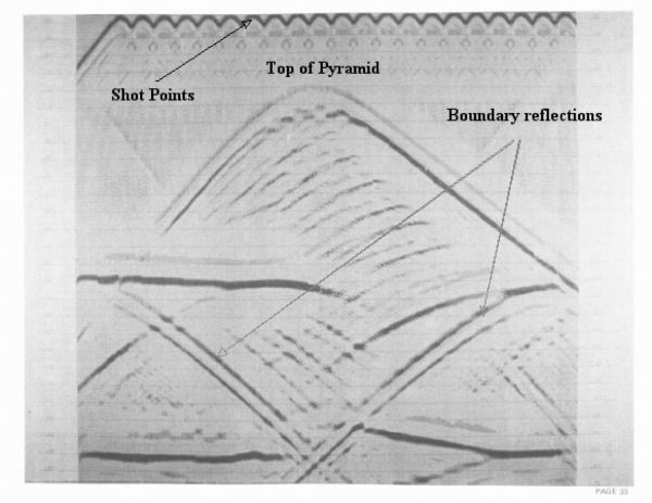
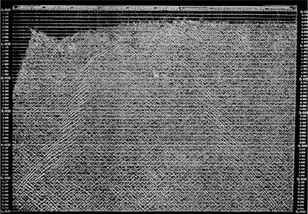
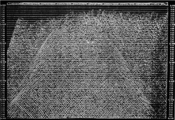
The shots in Figure  37 are from the pyramid model in Figure  38.

Figure 37: Shots 1-24 from the Pyramid model

Figure 38: The Pyramid Model

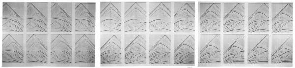
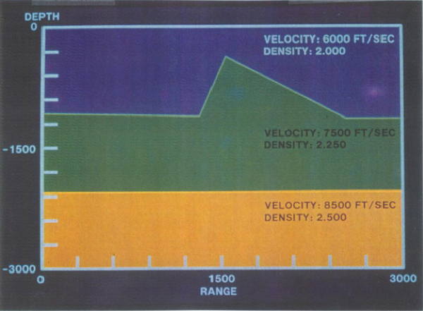
Figure  39 is a stack of the common-midpoint ordered data in Figure  37. NMO was performed using the root-mean-square velocity from the model used to generate the data. The "noise" in this data set is representative of a poor implementation of the approximations to the differential equation used to model the data. This kind of noise is related either to the fact that the differences have not been approximated well, or because damping at the boundaries is poor.

Figure 39: The stack of Shots 1-24 from Figure  37.

Figure  40 shows how dip affects arrival times as a function of half-offset.

Figure 40: Moveout for a dipping reflector.

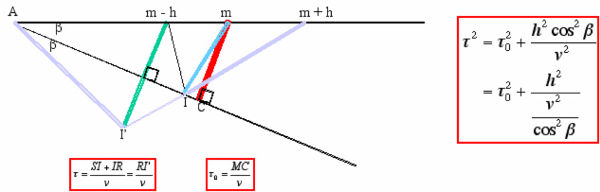
To relate the traveltime from source at m h ( S) to the image point, I, and back to the receiver at m + h ( R), note that in Figure  40, the length of the path from S to I and then to R is the same as the length from R to I 0. Using the law of cosines, we have Equation  8.

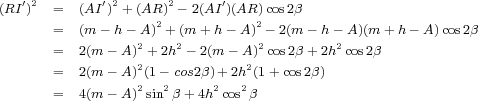
To get the time over the path from R to I 0, divide each side of Equation  8 by v ², as shown in Equation  9.

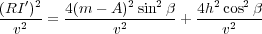(9)

Since the vertical traveltime is given by Equation  10, we get the final equation, Equation  11.

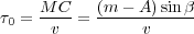(10)

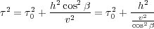(11)

The cosine term in the denominator of Equation  11 essentially increases the apparent velocity of the dipping reflector. For example, the apparent velocity of a bed dipping at 60 degrees will be exactly twice that of a flat reflector in the same velocity medium.

Figure  41 shows that reflections from a dipping reflector in a constant velocity medium appear to be from a flat reflector with a velocity of . The blue hyperbola is what actually defines the dipping event. The red curve is the hyperbola from a flat reflector with the same velocity, v.

Figure 41: The impact of dip as seen on a common-midpoint gather.

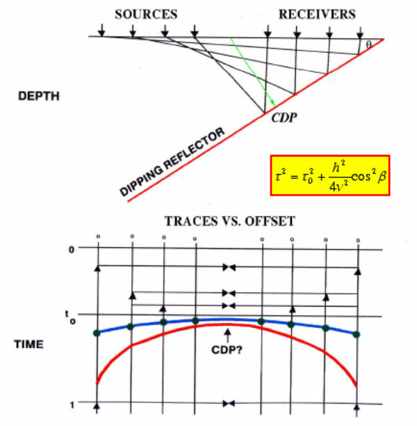
Note that for traces with a fixed midpoint, reflections from the dipping horizon do not correspond to a fixed common-depth-point (CDP) location (the intersection of the green line and the dipping reflector). In fact, the larger the offset between source and receiver, the greater the CDP-reflection point separation. This separation is referred to as CDP smear. To correct precisely for CDP smear requires that we prestack migrate the traces, since normal moveout will not work.

Nevertheless, the hyperbolic curve (blue in the figure) can still be corrected and stacked, it just cannot be stacked with the true velocity v, but must be stacked with the normally much faster velocity, v=. Thus, if we assume that the CDP smear is small, we could, in principle, stack the data with the faster velocity and produce some kind of representation of the dipping event. One way to do this, and then combine the dipping information with the standard stack, is to NMO with the faster velocity, filter out anything that is not flat, stack and then add the result back to the NMO stack.

Examples

To see how this might work, we will stack the data with velocities of the form v= _i over a uniform range of angles β _i, filter out anything that is not flat on the CDP gathers, and then stack.

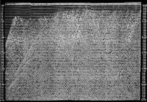
Figure  42 is an example stack of a two-dimensional Gulf of Mexico data set over an obvious salt structure. The process used to generate this unmigrated image was simply NMO followed by stack. There was no intermediate dip correction or migration.

Figure 42: A typical stack of a 2D data set from the Gulf of Mexico. This data was shot sometime in the 1980's.

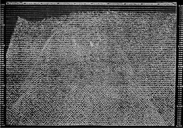
Figure  43 is a stack of a Gulf of Mexico salt structure using parameters and filters that attempt to image dip up from 0 to 15 degrees. What we actually did was find a set of velocities that we thought represented the sediment velocities, and then filter out all of the events that were over-corrected by normal moveout. Our best estimate is that the actual dips of the reflections comprising this image are no larger than 35 degrees.

Figure 43: Stack of the data in Figure  42 using an assumed dip of 7.5 degrees. At the bandwidth of these data the effect is to stack everything up to approximate 15 degrees.

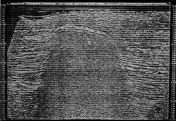
Figure  44 is a stack of a the Gulf of Mexico salt structure with parameters chosen to image events from beds with 15 to 30 degree dips. Note that what we are seeing are mostly reflections from beds whose dip is increasing as they approach the salt dome.

Figure 44: Stack of the data using an assumed dip of 22.5 degrees. At the bandwidth of these data the effect is to stack everything between 15 and 30 degrees of dip.

Figure  45 shows the stack of data over a Gulf of Mexico salt dome with parameters chosen to image reflections from events with 30 to 45 degree dips. As we increase the angle of the dips we are trying to image, we see that events reflected from more steeply dipping beds begin to appear. Again, this unmigrated image was produced by modifying the normal stacking velocity field to produce an apparent velocity field closely associated with dipping events in the 30 to 35 degree range.

Figure 45: Stack of the data using an assumed dip of 37.5 degrees. At the bandwidth of these data the effect is to stack everything between 30 and 45 degrees of dip.

By increasing the dip range to 45 to 60 degrees, Figure  46 shows that, in fact, there are reflections in this data set from beds that dip in excess of 45 degrees. What is more important is that these reflections cannot be seen in a typical stack which has not been dip-moveout corrected. Thus, if they are not imaged in a traditional stack, we cannot be expected to image them on post-stack migrated sections.

Figure 46: Stack of the data using an assumed dip of 52.5 degrees. At the bandwidth of these data the effect is to stack everything between 45 and 60 degrees of dip.

Figure  47 is a linear stack of the 15 to 60 degree dipping events. By stacking the sections from the last three figures, we get an idea of the events that should be in the original NMO-only based stack, but are not visible there. When these are migrated, a much clearer picture of the salt structure appears.

Figure 47: The sum of the sections in Figures 43 through 46.

Adding all of the sections together provides the final NMO-DMO corrected stack in Figure  48. This DMO corrected data set is much closer to a true zero-offset profile, and now includes reflections from steeply dipping events. Migration of this section will produce a much clearer picture of the salt structure.

Figure 48: The sum of the sections in Figures 42, and 47.

Remarks about DMO

In summary, correcting for dip using DMO partially migrates the data to address the fact that CDP arrival time curves have apparent velocities much faster than flat events. It converts upward sweeping hyperbolas in each and every NMO-corrected CDP into flat events at zero-offset traveltimes. Although it is possible to perform DMO using non-constant velocity fields, in practice, most DMO algorithms are constant velocity methods. They achieve their goals in much the same manner as an ordinary migration, but with much smaller operators. As seen in the earlier figures, it is possible to image dipping events using existing stacking and dip filter methods. What is even more surprising is that constant velocity DMO and even prestack time migration can be accomplished without knowing anything about the velocity.

The NMO-DMO-STACK combination is usually called partial prestack migration because it performs three of the four tasks involved in performing a prestack migration. After its application, the only remaining task is to position subsurface events properly. Because NMO-DMO-STACK is relatively cheap, this process played an important early role in improved imaging, and for a time became a standard part of every processing sequence.

However, since most DMO processes are based on constant velocity assumptions, or, at best, v ( z ) assumptions, they have considerable difficulty producing images below strong velocity variations. Thus, DMO-NMO is a useful tool for imaging steep dips, but is impractical when the objective is subsalt.

With the advent of inexpensive computers and the resulting ability to perform full prestack migration, DMO-NMO no longer reigns as the optimum approach to seismic imaging.