Raytracing

For a source at x _s and receiver at x _r, if we denote the traveltime or phase from x _s to x _r by φ ( x _r ;x _s ), and the Amplitude decay by A ( x _r ;x _s ), we can then write Equation  147 in space-time and Equation  148 in frequency.

(147)

(148)

Substituting into the wave equation in Equation  149, we get Equation  150.

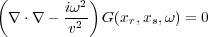(149)

(150)

Equating coefficients of powers of iω to zero yields the Eikonal equation, Equation  151 and the transport equation, Equation  152.

(151)

(152)

Simultaneous solution of Equation  151 and Equation  152 provides the traveltimes and amplitudes necessary to approximate the Green's function in an efficient manner. While not straightforward, the Eikonal equation as specified here can be solved by finite differences and/or the method of characteristics. The method of characteristics is usually referred to by the more traditional raytracing label.

The method of characteristics is so called because it solves the Eikonal equation along rays by simultaneously solving Equation  153 and Equation  154.

(153)

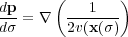(154)

In this case, σ typically represents arc length along the characteristic or ray, and x ( σ ) is the position of the ray vector at the distance σ from the initial position of the ray. The process is usually initialized by setting x (0) = x _s to the initial source position and setting, as shown in Equation  155.

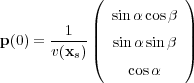(155)

Once x ( σ ) is known, the desired traveltime is computed by integrating along the characteristic curve in Equation  156.

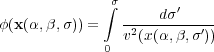(156)