Granitic Overthrust

Figure  11 shows a granitic overthrust model from the Northern United States together with a simulation of a zero-offset section using that model. The problem is to unravel this data and put it back in its proper location. The objective are the sediments below the granite thrust.

Figure 11: A Granitic overthrust example from the state of Wyoming in the United States of America.

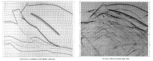
Granitic overthrusts are certainly as difficult to image as salt structures. Granitic structures are representative of structures with velocity contrasts between 3 and 3.6 to 1, where granite velocities are usually between 6800 and 7000 m/s, while near surface velocities are in the neighborhood of 1800 m/s.

Imaging the top and base of such structures with a time migration is almost impossible.

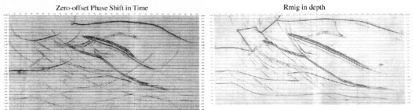
Figure  12 shows that a comparison of phase shift migration with reverse time migration is in reality no comparison at all. A single velocity function simply cannot cope with the extreme variation in the actual Earth model.

Figure 12: Phase shift versus full two-way-reverse-time migration.

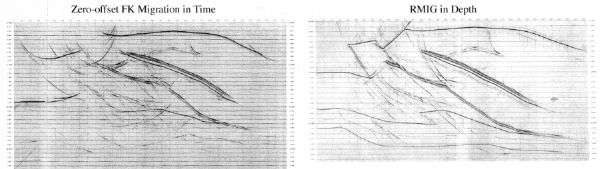
Figure  13 shows that an FK migration is no better than the phase shift of the previous figure.

Figure 13: FK versus full two-way-reverse-time migration.

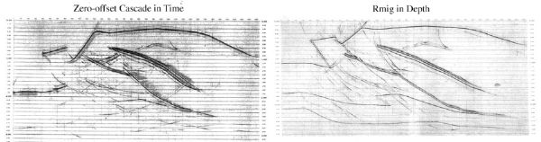
In contrast to the previous methods, the cascade migration shown in Figure  14 does a superior job of imaging above and to the left of the granitic intrusion, but simply cannot image anything below the granitic overthrust accurately.

Figure 14: Cascade versus full two-way-reverse-time migration.