Huygens Principle and Integral Methods

One of the most powerful seismic modeling concepts, known today as simply the Huygens Principle was expressed some 350 years ago by both Christiaan Huygens and Augistin Jean Fresnel:

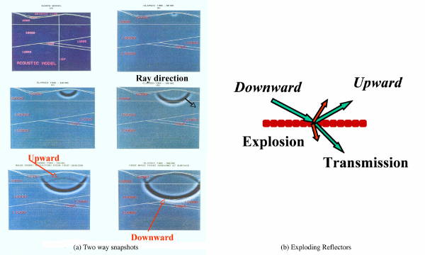
While we frequently drop his name and simply call this Huygens Principle, Fresnel's contribution cannot be minimized, but the part we really need to understand is visualized in Figure  33. This principle is usually explained conceptually by saying that the way Huygens arrived at it was based on observations of what happened when he dropped a finite number of balls, N, into the Zuider Zee. When the balls were arranged in a line, what he saw was not N independent events, but something more akin to a moving line. He saw the envelope of the wavefields as opposed to the independent wavefield of each separate ball. That being said, it is much more important to think in terms of the formal discussion above. Perhaps a better example of Huygens/Fresnel Principle would be to recognize that a discussion in an adjacent room would actually appear to come from the connecting door. Clearly, the door is acting as a new source term and the entire sound volume appears to the observer to come from that source. Figure  33(a) shows this for two-way waves and emphasizes that fact we need not think of a single reflector. Parts (b) and (c) of this figure show what happens when waves are allowed to travel in only one direction.

Figure 33: A simple graphical interpretation of the Huygens/Fresnel Principle.

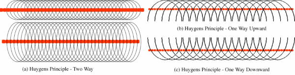
We see that the wavefield due to a reflector, the red flat line in parts (a), (b), and (c), can be thought of as the envelope of an infinite series of point sources. Each point source can be thought of as having been ignited by an impinging wavefront which in part (a) results in both a reflection and a transmission. Parts (b) and (c) visualize what happens when propagation is only allowed upward (b) or downward (c).

One of the more mathematically complex ways to use this principle is to recognize that regardless of the type of media (acoustic, elastic, or anisotropic), we can think of the total response of any give source in terms of what happens at any given point in the actual model. For example, a source on the surface eventually arrives at some point ( x;y;z ) with reflectivity R ( x;y;z ). According to Huygen's principle, the energy of the source then generates a virtual source at ( x;y;z ), the energy from which then propagates through the entire model, and then perhaps to receivers on the recording surface. In a nutshell, what this really means is that we need only know the response of each point in our model to completely reconstruct the entire wavefield u ( x;y;z;t ). 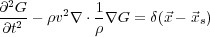For the pressure formulation, this concept is mathematically expressed in terms of the so-called Greens' function G ( ; _s ;t ) as shown in Equation  139, where = ( x;y;z ) is a generic point in the medium and _s is the vector location of the source.

(139)

For a given source, s ( ₀ ;t ), integration by parts allows us to express the solution p of Equation  17 in the integral form of Equation  140.

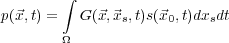(140)

What we are saying is that the solution to the equation is just the sum of all the point responses of the medium under consideration.

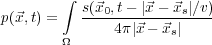
For example, when the velocity and density are constant, the Green's function takes the form in Equation  141 and Equation  142.

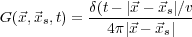(141)

(142)

Thus, p ( ;t ) is the superposition of all the point responses in the medium due to a source at the point ₀ = ( x ₀ ;y ₀ ;z ₀ ). Another way to say this is that the Green's function G is the inverse of the operator in Equation  143.

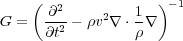(143)

Scattering

In integral form, these formulas lead to what has become known as Domain-Integral Methods for solving seismic scattering problems. These methods have not been popular for seismic modeling so they are only of passive interest for us. They are important because they divide the seismic propagation scheme into incident and scattered parts. In theory, the ideas can be based on any of the equations above, but for illustrative purposes, we only consider the pressure case when the density is constant. The basic idea is to assume that the velocity v can be expressed as the slowness difference = , where c ₀ is constant. We can then write Equation  144, so that our solution takes the form of Equation  145, where p ^inc is defined by Equation  146.

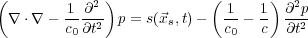(144)

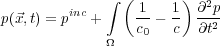(145)

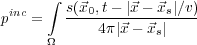(146)

Although a bit of a stretch, Figure  34 illustrates Huygens' principle in considerable detail. Here we see the wave reflections and transmissions at each point in a given medium.

Figure 34: Wave directions and exploding reflectors.