Shot Profile Prestack Migration

Shot profile migration is a process by which each shot record is migrated separately and the result is summed into the final image volume. This process is sometimes also called common-shot migration or just shot migration.

Performing Shot Profile Migration

Shot-profile migration consists of three steps. In the first step, a synthetic shot is generated and propagated into the Earth. In the second step, receiver traces are reversed in time, used as sources in the modeling code, and then downward continued into the Earth. The third step forms an image at each depth or time slice through the application of an appropriate imaging condition.

This three-step approach is based on what is known as the cross-correlation method and was popularized by Jon Claerbout (1971, 1986). Figure  3 conceptualizes the basic ideas. The left hand side of this figure represents the forward propagation of the shot into the Earth, while the right hand side shows the backward propagation of the traces corresponding to this shot. In this figure, shot synthesis is generating a downward traveling wavefield, while the backward propagation of the receiver traces is generating what ultimately becomes an upward traveling wavefield.

Figure 3: Migration of common shot profiles

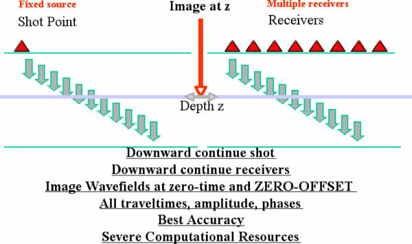
Note that we can choose virtually any pair of modeling algorithms for the basis of shot-profile migration. When a full two-way approach is used for both the shot and receiver steps, the result is a full two-way algorithm. When a one-way wave equation is used for both the shot synthesis and receiver back-propagation, the result is definitely a one-way method. Of course, it is possible to use two different modeling methods. We could use a raytrace-based method for the shot synthesis and a full two-way back-propagation for the time-reversed receiver traces. Virtually any combination of the modeling algorithms discussed in Chapter 2 is possible, so the number of prestack shot profile methods is quite large. We will avoid giving these hybrid methods names, but we will attach names to methods for which the shot synthesis and receiver back-propagation methods are algorithmically identical.

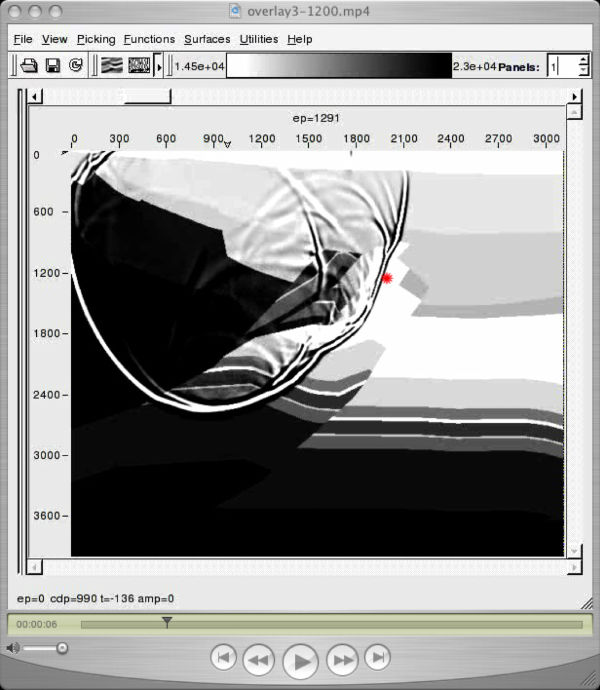
Understanding shot-profile migration is mainly dependent on comprehension of the third (imaging-condition) step of the shot-profile migration methodology since the modeling pieces are straight forward. To help understand the imaging condition, recognize that, as shown by the red dot in the movie corresponding to the image in Figure  4, each subsurface image point can be thought of as a seismic receiver that records signals from both the source and the receivers. The trace from the downward traveling source wavefield registers no arrivals until the first source amplitude arrives after τ _S seconds. This, of course, is the time it takes for energy from the source to ignite the virtual reflector at the image point.

Figure 4: A wavefield arriving at a subsurface image point (in red)

An example of such a trace showing two arrivals recorded from a source is shown in the top trace in Figure  5. An example of a second trace showing three arrivals from the backward propagated receivers is shown in the bottom trace. Because it was generated from time-reversed traces, amplitudes at the longest time are due to amplitudes recorded at the maximum recording time, τ _max. After backpropagating for τ _{max S} seconds, the full wavefield that radiated out from the image point as it acted as a virtual source has arrived at the receiver located at the image point. At this time stamp, there are still τ _S seconds left to propagate, but none of these amplitudes will be recorded at the image point. Thus, both traces contain exactly two arrivals. Imaging is accomplished by summing all the amplitudes in a a point-by-point multiplication of the two traces and then adding the result to the image point location. In graphic detail, this is exactly Jon Claerbout's cross-correlation imaging condition (1971, 1976).

Figure 5: Downward (source) and Upward (receiver) arrivals at a subsurface image point

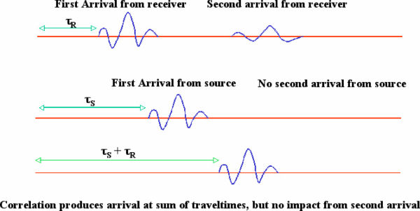
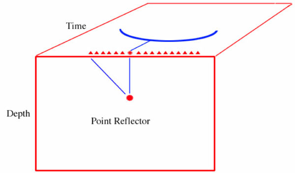
Figure  6 is a further attempt to clarify Claerbout's imaging condition. This figure shows a subsurface model with a single point reflector in red on the face and the time section indicated by the blue arc on the top. It contains three potential point reflectors indicated by two black dots and one red dot. The red dot is the only point reflector in the model.

Figure 6: Point reflector response with forward source and backward receiver wavefields at two subsurface locations.

We see that events on the two recorded traces do not overlap at the upper black image point. Thus, applying the imaging condition produces zero amplitude and no reflectivity, as predicted, and no point reflector is detected. On the other hand, at the black dot that is near the red point reflector, the events on the two traces may be close enough to the red dot to produce a small amplitude, and as a result the point reflector begins to be detected. Claerbout's imaging condition is just the ticket for detecting the only point reflector in the model.

It may not be surprising that there was more than one arrival in each of the two traces at the image point. As indicated in the propagating wavefield in Figure  4(a), multiple paths from the source location to any subsurface image point is probably the norm in complex geology. In spite of that, it is important to recognize that there are several algorithms that make the surprising assumption that only one arrival is present at each subsurface location. We will see that single arrival methods, while useful, are very sensitive to the kinds of velocity variations seen in even relatively simple geologic settings.

As was the case on historical approaches in Equation  3, migration was performed by hand on a shot-by-shot basis. In that case, the imaging was based on direct estimation of local dips coupled with a crude velocity guess. To emulate this process using our modeling methods, it was necessary account for the propagation from the source to the reflection point, and from the reflection-point to the receiver for each and every trace in our survey. This was accomplished by a forward shot propagation and a backward propagation using the recorded data reversed in time as sources. Clearly, both steps could employ exactly the same modeling code. The only real difference between the two is that one used synthetic source data while the other used the actual recorded data in reverse time order. Do not be discouraged if this does not seem simple or intuitive. In 1971, very few practicing geophysicists thought anything like this would ever be possible and many thought Claerbout's method would never be practical. They were wrong.

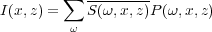
In precise mathematical terms, Claerbout's time-coincident imaging condition is mathematically represented by Equation  1, where I ( x;z ) represents the seismic amplitude at the position ( x;z ) in space and depth, S ( t;x;z ) is the downward traveling source wavefield, and P ( t;x;z ) is the backward-propagating seismic-shot record.

(1)

In this case, is interpreted to mean cross-correlation and ) t = 0 means to evaluate at zero time for this depth. This process usually takes place in the frequency domain, so evaluation at time zero just means to sum over frequency. In this case, the formula is given by Equation  2.

(2)

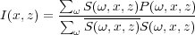
Refinements to this simple process abound. One of the simplest improvements, is given by Equation  3.

(3)

This improvement in the frequency domain normalizes Equation  2 by the spectrum of the source wavefield. Because the source wavefield is what illuminated the subsurface in the first place, dividing by this value has the general affect of correcting for uneven illumination. It generally results in improved amplitude preservation, but should not be considered as the final word in amplitude preservation.

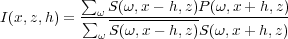
When the velocity field is exact, the imaging condition, as described by equations 1 and 3, produces sharp and accurate maps of subsurface reflectivity. When the velocity field is incorrect, many point reflectors may not be imaged or may be imaged very poorly. It is quite natural to ask if there is some modification to the image condition that might make it possible to assess the accuracy of the velocity field or even to produce a method to estimate velocity corrections. One answer to this question is given by the non-zero offset imaging condition in Equation  4, and the other by the time shift zero offset condition in Equation  5.

(4)

(5)

In Equation  4, h is a scalar with units of feet or meters at depth that measures where the two wavefields achieve maximum lateral correlation. It defines a range of subsurface offsets that, in principle, offers the possibility for sensing and correcting for velocity errors. When the migration velocity is incorrect, the best image will appear at some positive or negative h. How far the wavefields are separated can be used to estimate a new velocity volume or field.

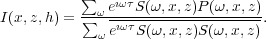
In Equation  5, τ is a scalar at depth with units of time that tells us how close the two wavefields are in time at depth. The scalar τ is not directly related to surface time; it is merely a value indicating the difference between forward source and backward receiver times. Instances where non-zero τ's produce the best image are indicative of inaccurate velocities and the value of τ becomes useful in estimating a new velocity field.

It is worth noting that both of these approaches can be converted to methods that produce gathers parameterized by opening or reflection angle and azimuth in 3D. The mathematics are beyond the objectives of this book, but these migration angle gathers can be analyzed in much the same way that more traditional offset gathers are currently used to estimate subsurface velocities.

In the frequency domain, equations 4 and 5 have the forms in equations 6 and 7.

(6)

(7)

Shot Profile Migration Example

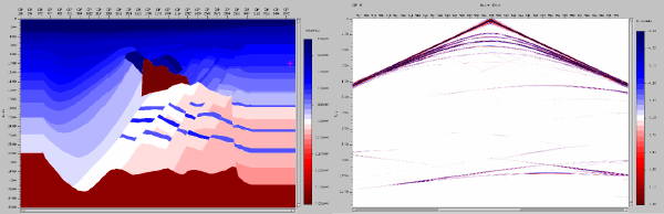
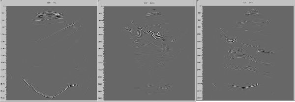
The black lines in Figure  7(a) show the location of three shots with receivers spanning the entire model. Part (b) shows one-way shot profile migrations of these shots. Note that each migration images a substantial portion of the subsurface. These images were actually produced using the imaging condition of Equation  3. Thus, the process included approximate correction for illumination.

As noted earlier, every algorithm in Figure  1 can be used as part of a shot profile style migration method.

• Pure XT algorithms are either one-way or two-way and are usually implemented using finite difference approximations.
• Of the FK methods, only the PSPI method is popular.
• The most popular one-way method is based on the FKX phase screen method of Ru Shan Wu and colleagues, or on methods that are slight variants of this technique.
• Plane wave modeling techniques are also in demand because they can be applied very efficiently.
• In contrast, raytrace (Kirchhoff) shot-profile approaches are not popular because this method is usually implemented to image common-offset volumes rather than shots. This structure facilitates the production of common-offset image gathers, and their use directly affects estimation of interval velocities.

Combinations of these methods are rare. Some that probably should have received attention include combinations of Gaussian Beam and two-way-reverse-time, as well as Gaussian Beam and one-way-phase screen or PSPI.