Zero Offset Hand Migration

Given records like that in Figure  2, early explorers made a stickmap that might have looked something like the one displayed in Figure  3. The times defining the event in this figure would most likely have been based on the identified arrival from the closest trace to the shot point. They would have liked to have a trace in which the shot and receiver were coincident. But, because they were using dynamite, this would have resulted in the destruction of the receiver, and so they settled for receivers that were close to the shot. In Figure  2, the closest trace would have been the time pointed to by the arrow with a shot-receiver separation (offset) of about 100 meters. This separation would have to suffice as an approximation to a trace with coincident source and receiver. Such traces were called zero-offset traces.

Figure 3: A simple non-flat horizon.

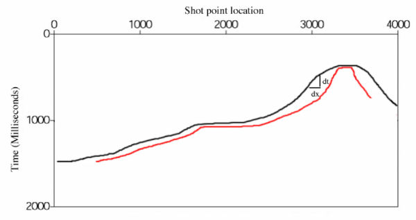
The black line graph in Figure  3 represents what is called a zero-offset or unmigrated time section. What is necessary for exploration and drilling is a depth map, or, when the velocity is constant, a migrated time map as conceptualized by the red line graph. In this case, the red line was simply drawn in free-hand, but represents the major features of what might be the true migration position of a reflected horizon. Note in particular that after migration, the peak of the anticline has not changed position, but its width has shrunk. It is also true that the positions of all dipping events have moved up-dip in every case.

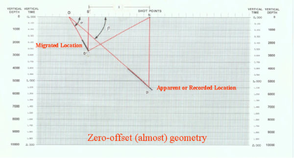
To produce the red-line section in Figure  3, we need to know how to convert unmigrated arrivals into migrated arrivals. Figure  4 shows the relationship between zero-offset reflections and their correct migrated position. The true reflector has a true dip angle of α, while the apparent or recorded event is at dip angle β. In this figure, the data is assumed to have been recorded over a constant velocity medium. Note that the location of the migrated event is placed relative to vertical time or depth, but remember that this vertical positioning is only valid for constant velocity media. Since the velocity is constant, vertical depth is given formally by the traditional relationship, where depth is equal to velocity times one-way time, that is, d = vt= 2 or t = 2 d=v.

Figure 4: Fundamental migration geometry between the apparent location and dip β versus the migrated location and dip α.

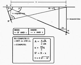
Migration in a two-dimensional, constant velocity medium requires only that we know the sound speed in the medium, and can measure the ratio of the change in arrival time to the corresponding horizontal change. As indicated in Figure  5, this is usually specified in seconds per trace divided by the trace spacing, but any time interval and corresponding spatial interval will do. The formulas listed in the figure provide all necessary calculations to determine the migrated position of any given event. Note again that in this simple medium, vertical depth is easily obtained by multiplying the vertical time, t, by the medium sound speed, v. Note also that events with any given apparent dip migrate up-dip. Consequently, we can ignore the sign of any given value and simply place the migrated dip element at its appropriate up-dip position. As we will see, extension of this formula to a vertically varying medium is quite easy.

Figure 5: Fundamental migration trigonometry relating the apparent location and dip specified by S and β versus the migrated location and dip specified by S 0 and α.

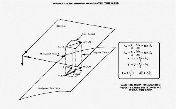
Figure  6 extends the migration formulas in Figure  5 to a three-dimensional constant-velocity medium. These equations provide the necessary computational formulas to complete the migration process. Here, however, it is a bit more difficult to actually do the migration by hand. At this point, the migrated position must be contoured to produce a migrated map of the recorded event.

Figure 6: Fundamental migration trigonometry relating the apparent location and dip specified by the S and β versus the migrated location and dip specified by S 0 and α.

Beginning in the late 1940's and continuing until the early 1960's, all interpreters used this approach to produce migrated prospect maps. The equations were employed in a two step manner, where calculations proceeded in the line direction, and were then followed by similar calculations in the cross-line direction.

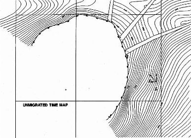
Figure  7 shows an example of an unmigrated or zero-offset map. In this case, faults and the large truncation surrounding a large salt dome are clearly evident. This map is from an early interpretation done over a salt dome in the Gulf of Mexico at South Pass Block 89.

Figure 7: An unmigrated (zero-offset) time map of a salt structure in the Gulf of Mexico. This particular map was contoured in 1972 or 1973 from a two-dimensional grid.

The vectors graphed in Figure  8 are the result of using the equations in Figure  6. A computer was used to generate and plot the vectors. Note the significant change in the shape of the salt structure and note also that some of these vectors are over two miles in length. It is important to observe that any 2-D migration of the red line will be inaccurate. Not only does its subsurface position migrate up-dip, but its shape can change quite dramatically. This is a fundamental reason why 3D imaging is so superior to 2D.

Figure 8: Migrated vectors from the map in Figure  7 computed using the formulas in Figure  6.