Velocity Independent Prestack Time Imaging

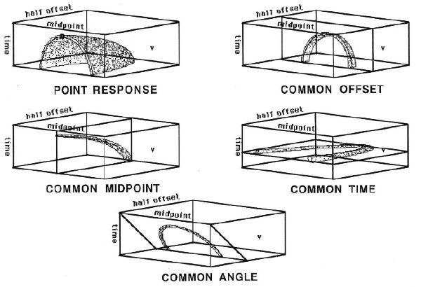
Figure  14 shows various slices through the seismic response for a point reflector in a purely constant velocity medium. The top left figure is the response due to a single point reflector. Proceeding in a counterclockwise manner, we see a common-depth point slice, a radial or common-angle slice, a common-time-slice, and finally in the upper right, a common offset slice. In this constant velocity world, it should not be difficult to envision a method for imaging each of these particular orientations of the data.

Figure 14: Point response in a constant velocity medium

Common-offset sections actually look like normal stacked seismic sections, but there is a difference. In the near offset on the left side of Figure  15, the section closely resembles a normal stack, while the far offset on the right appears to be a squeezed version of the section on the right. Even though these sections are from the two dimensional anisotropic model in the lower right hand corner, anisotropy is not really visible to the naked eye. Moreover, traditional normal moveout correction, even though it supposedly stretches the data to equivalent zero-offset time, will not ultimately produce anything close to a true zero-offset stack.

Figure 15: Near and far offsets

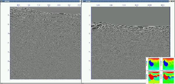
Figure  16 details an unusual methodology for imaging or migrating data in constant velocity media. It combines what we have learned in the previous figures to allow us to image the point source response while delaying the velocity analysis until the very end.

Figure 16: Dip independent prestack imaging

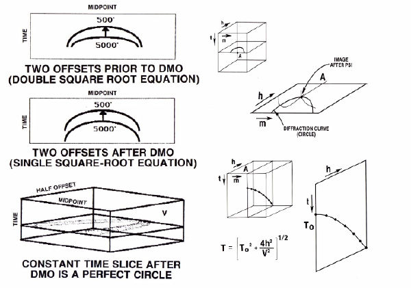
The left hand side of this image essentially shows what happens when we apply DMO. The top graphic shows the input data from a single point source. That is, it represents two different common-offset slices superimposed on one another. The middle figure on the left hand side shows the same two offset slices after DMO. Note that, in this case, the two common-offset images differ only by moveout time. In the bottom part of the left hand side, we see that, after DMO, any time slice appears to be a circle. That being the case, we can image this circle to a point by simply migrating it as in the previous figures. Once this is done, as indicated by the top figure on the right, we will have reduced the point source response to a single CDP whose moveout velocity provides the necessary information to image the point at its correct subsurface location.

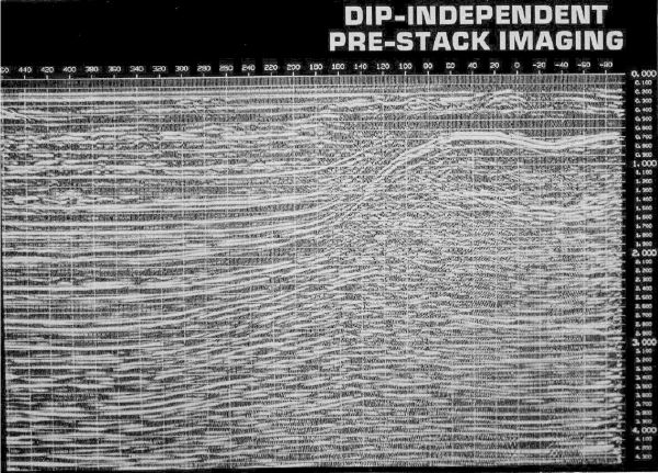
The completely velocity independent prestack imaging method that produced Figure  17 delayed velocity analysis until the very end of the process. This means that the velocities obtained from this approach are actually migrated velocities, and consequently are measured almost vertically. The importance of this statement is that this set of velocities are much more consistent with the assumptions made to ensure the accuracy of the traditional Dix vertical inversion scheme.

Figure 17: Application of dip independent prestack imaging in the Gulf of Mexico