Depthing

Geophysical approaches to finding vertical velocity fields abound. Some of the earliest were called depthing, or, perhaps more precisely, depth conversion. Depth conversion typically begins with a careful analysis of the wells of interest.

Figure  5(a) shows how the overburden above the potential reservoir is separated into different velocity units. Starting at the surface, we model the velocity behavior in layer 1 and create a depth map for horizon 1. We then model the velocity in layer 2 and hang the depth conversion from the depth horizon we already have for horizon 1. We repeat the process for each layer until we reach the maximum depth desired.

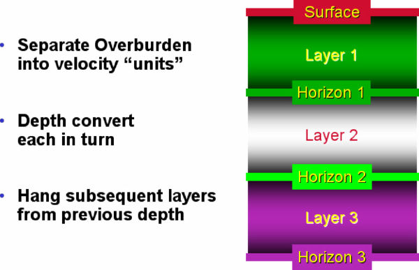
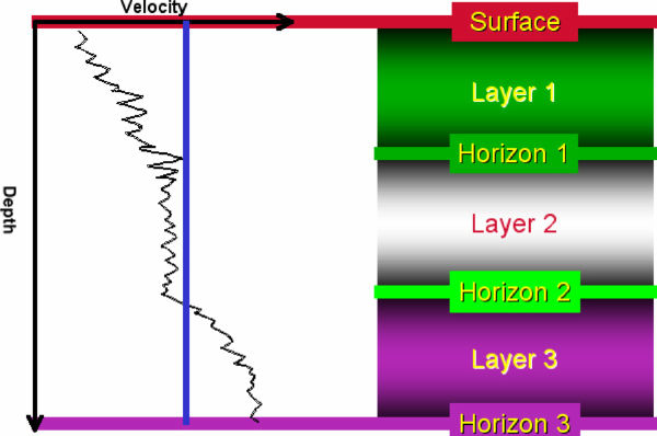
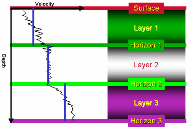
Figure  5 shows the typical approach to analyzing wells to determine a well or depthing velocity structure. The graphic in (a) of this figure presents the standard process. The well is separated into overburden units or well tops of horizons of interest. Each of these units can then be converted to depth. Analysis of each such unit can be simple, as indicated in Figure  5(b), or more complicated as indicated in (c) and (d). The more accurate approach is clearly represented by Figure  5(d).

Depending on the complexity and strength of the velocity variation within the well, we can minimize the number of depth units. Figure  5(b) shows the simplest technique using a single average velocity. We ignore the layering just described, and compute an average velocity from the surface to the target horizon. This has the advantage of being simple and quick to implement, but has the disadvantage that, since the behavior of the subsurface is not fully modeled, our confidence in the predictions may be reduced. This is a good domain for viewing stacking velocities, because they have seen all of the overburden anyway.

Moving to a more sophisticated approach in Figure  5(c), we look at interval velocity. Here, we assign a constant velocity to each layer. This velocity may vary spatially from well to well. We can model this by cross plotting interval velocity versus midpoint depth, for example, or we can contour the well interval velocities, perhaps geostatistically using our seismic processing velocities as a guide.

An even more sophisticated approach, as shown in Figure  5(d), is the use of instantaneous velocity functions. Here we are modeling the detailed velocity variation with depth on a layer-by-layer basis. The most commonly used relationship is the linear increase of velocity with depth (the V0Kz method), although modern software packages can handle any function, as shown in the third layer. Any of the parameters in these equations can be represented by grids, thus allowing full flexibility.

Constructing complex horizon-based models can be quite difficult. Figure  6 illustrates several requirements for different geological settings. What is important is to recognize that in a horizon-based model building exercise, we must interpret many more horizons than is usually necessary for exploration purposes. Moreover, many of the additional horizons have zero prospectivity and, consequently, are of little interest to interpreters, although these layers can be extremely important for depth imaging.

Figure 6: Complex model construction

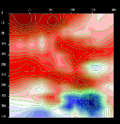
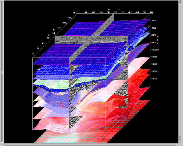
Horizontal velocity trends are thought to be linked with vertical velocity trends. Thus, using trends from the prestack depth migration velocity analysis can be used to statistically interpolate sparse well data sets. Figure  7 is an example velocity slice from a seismically derived Earth model. It could serve to define trends for extrapolating sparse wells to construct a detailed well field.

Figure 7: Seismic derived velocity slice.

Horizons, like those in Figure  8(a), can be used to guide the interpolation process in a horizon consistent in a lap or off lap manner. If we decide that the subsurface geology follows the structure defined by the given horizons, a suitable projection of this estimated velocity functions on to a grid of locations defined by the user will produce a structure tracking velocity field.

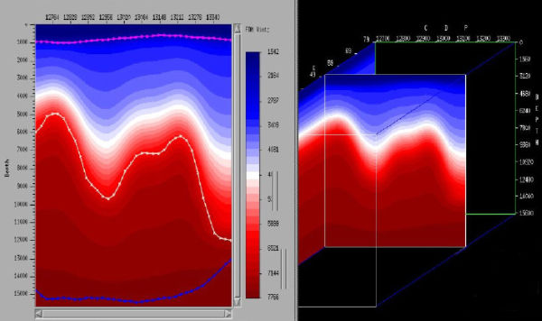
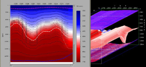
In Figure  8(b), a single well, at the location indicated by the arrow, is interactively projected into the three-dimensional grid. After projection, we have logs at an evenly sampled grid of surface locations, Figure  8(c). In this case, projection was based on shrinking and stretching the single input function to track the given horizons.

Figure  8(d) is a slice through the projected well field, while Figure (e) shows RMS velocities calculated from the well field. In a sense, this process reverses the usual process of estimating interval from RMS velocities. Figure (f) is a contoured version of (d) showing how the actual projection was performed.