Semblance-Based Isotropic MVA on CIGs, CAGs, and SMIGs

Figure  10(a) shows common input offset image gathers generated by migrating each input sorted offset with a most energetic arrival Kirchhoff algorithm. Figure  10(b) shows common azimuth generated common angle gathers and associated common angle semblance panels. The angles range from 0 to 60 degrees in increments of 2 degrees.

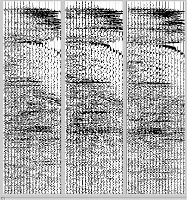
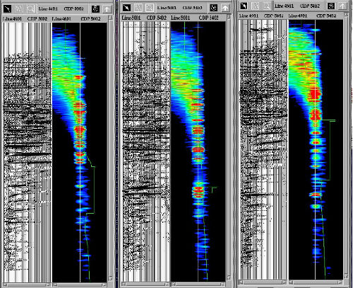
Figure  11(a) visualizes the kind of information angle gathers provide in sediments as compared to subsalt settings. In (a), the general loss of angle information is gradual as depth increases. In contrast, (b) shows that the loss of angle information below salt (or any high velocity anomaly) is quite dramatic. This is one reason angle gathers might be preferred over other forms of velocity analysis.

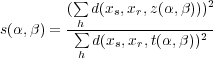
The velocity analysis/inversion formulas for estimating velocity models from either offset or angle gathers are shown in Figure  12. Note that the difference occurs because, in the old case, the method estimates velocity without any knowledge of the velocity used in the migration process, while in the new case, that information must be available. Regardless, both methods are based on producing a maximum energy or semblance display that can be directly picked to refine velocity estimates.

Figure 12: Angle Gather Velocity Analysis

Whether we use

(1)

or

(2)

estimating v is usually based on semblance panels calculated from Equation  3 or Equation  4.

(3)

(4)

In this case, s is bounded between 0 and 1, but velocity at any given t or z is taken to be the value that maximize the semblance. In spite of the fact that theory underlying these equations assume flat lying reflectors, they have proven to very useful in development of seismic imaging velocity models for both time and depth imaging.

Figure  13(a) includes images of a depth-to-time converted SMIG, a semblance panel computed from the SMIG, the current section under analysis, and the velocity model under construction. The process of actually doing the velocity estimation is shown in Figure  13(b). From left to right, we see the raw depth-to-time converted SMIG and semblance panel, the picked SMIG with hyperbolic trajectories and semblance panel, and the moveout SMIG with semblance panel. This figure confirms that SMIGs can be used for migration velocity analysis and also demonstrates the current semblance based analysis process for developing short-spread velocity models.

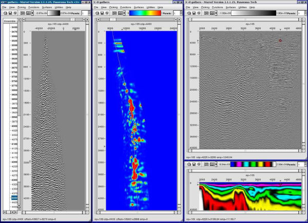
Figure  14 compares a common-midpoint gather, a common-midpoint gather with DMO, and a Kirchhoff depth migration common-image gather to assess the impact of partial and full migration, at least visually. The red line in the DMO stacks in (a) and (c) indicate a location where a CIG was selected for comparison. Part (a) is from an area where subsurface horizons do not dip severely, while Part (c) is from an area where subsurface horizons do dip severely. If our interpretation of the theory is correct, there should be little change in our velocity picks at (a), but considerable change for those at location (d). Changes from stacking velocity to DMO stacking velocity to migration velocity picks should be minimal in the former case and much more noticeable in the latter.

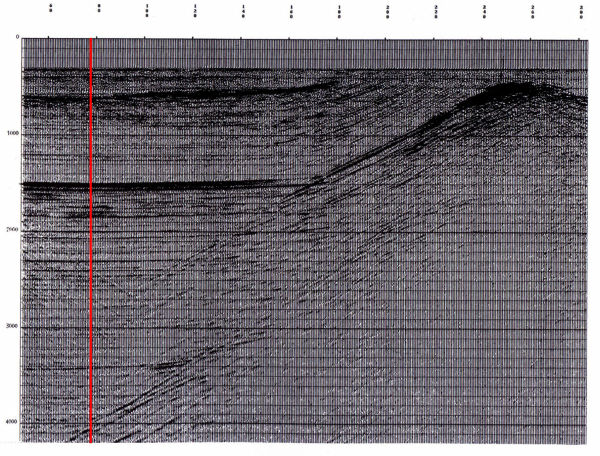
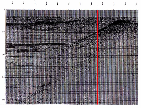
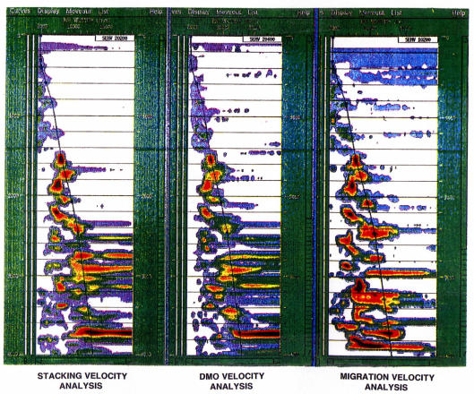
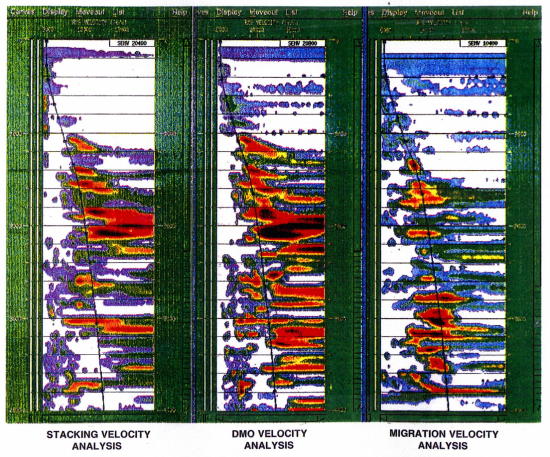
Figure  14(c) shows the picked curve from the migration analysis panel in (a) overlaid on the DMO panel and stacking velocity semblance panels. Note that while the panels differ in character, there is little reason to change the overall set of picks from one panel to the other. The theory seems to be reasonably solid when the horizons are flat.

In contrast to Figure  14(c), the picks in the panels in (d) are significantly different from each other. Even the DMO corrected panel in the middle, while better, is still significantly different from the Kirchhoff migrated common-image gather. We would certainly be inclined to argue that stacking and DMO based velocity estimates are inferior to those obtained from this Kirchhoff based depth migration algorithm.

Figure  15 shows the result of three iterations of what we will ultimately call the painless approach to velocity model building. No horizons were used to estimate the migration velocity. While more modern migration algorithms may produce improved images, the common-image gathers are flat, and, in spite of the inability to image the base of salt, the process clearly works, even in areas where the geology is complex and the rocks are hard.

Figure 15: Full prestack depth migration of the Barents Sea data.