Partial Prestack Migratio–Azimuth Moveout (AMO)

Except for pure land acquisition, it is generally very difficult to record pure common offset or pure common azimuth data. Economics limits such recording on land, and cable feather makes marine acquisition of such data almost impossible. Consequently, methods have been developed to map recorded data into the proper framework. Azimuth Moveout (AMO) is one such approach. As defined, AMO is the combination of DMO to zero offset, followed by inverse DMO to a fixed non-zero offset. Figure  8 is a revision of Figure  30.

Figure 8: Constant velocity non-zero offset equal traveltime curve.

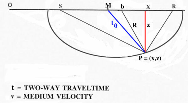
With a little bit of Greek mathematics, it shows that the time, t, of the equal traveltime curve in a constant velocity medium satisfies the elliptical equation in Equation  8, where, of course, t is the traveltime from S to P to R, and h = ( R S ) = 2 is the half offset.

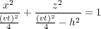(8)

It is interesting to determine the time, t ₀, in terms of v, t, and h, but doing so is not completely straightforward mathematically. What we first need to recognize is that t ₀ in Equation  8 lies on the circle defined by Equation  9.

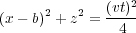(9)

For readers with a bit of calculus, if we take the derivatives of Equations 8 and 9 with respect to x, we get, respectively, Equation  10 and Equation  11.

(10)

(11)

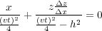
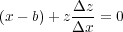
Note that Δz = x is the slope of the local tangent or, more practically, the slope of the reflecting migrated event if P was its location. Using Equation  11 to eliminate Δz = x from Equation  10 yields Equation  12.

(12)

After simple algebraic manipulations, the result is Equation  13.

(13)

What this formula tells us is that the zero-offset time, t ₀, is a function of the offset, h, the velocity, v, and the traveltime, t. A key point is that t is the input time on the input trace and t ₀ is the zero-offset time. What we want a DMO process to do is to map data at time t to data at time t ₀. A bit of trickery due to D. Forel and G.H.F. Gardner (1986) makes this possible. What they wanted after DMO processing was a data set that satisfied an equation of the form in Equation  14 for each new offset k.

(14)

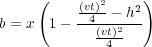
They realized that, given t ₁ and k, they could rewrite Equation  13 in the form of Equation  15.

(15)

Then, if they chose k ² = h ² b ², the result would be Equation  16, which simplifies to Equation  17.

(16)

(17)

Thus, all DMO amounts to is a simple mapping from offset h and time t to offset k and time t ₁. Moreover, this mapping is entirely velocity independent. This means that DMO and, consequently, DMO inversion can both be performed in a completely velocity independent manner. Forel and Gardner also realized that this process can be carried out by replacing each input trace with an ensemble of output traces having offsets determined by k through b and time specified by t ₁.

Figure  9(a) shows an ensemble of replacement traces for DMO on the left and DMO inverse on the right. As we might expect, what we see are smiles for the former and frowns for the latter. Figure  9(b) shows what happens to a purely inline common-midpoint gather after DMO is applied. Note that, after DMO, the source-receiver axis is orthogonal to the input source receiver axis. If we apply DMO inverse to the DMO'd data, the result would be to simply rotate back to the original orientation.

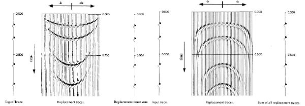
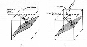
Figure  10 shows how to modify AMO (DMO followed by DMO inverse) to achieve an output source-receiver orientation of any desired angle. DMO is first applied along the output trace orientation indicated by the h _O vector in part (b). DMO inversion is then applied orthogonally to this direction. This process transforms an input volume with virtually random azimuths into one with a fixed azimuth and with only four dimensions.

Figure 10: Arbitrary angle AMO

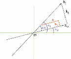
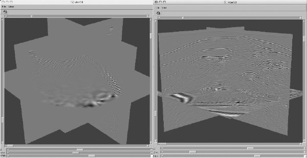
Figure  11 shows an AMO impulse response on the left and a full 3D volume on the right. The input trace from the SEG/EAGE C3-NA synthetic data volume used for the impulse response had an azimuth of -2 degrees and an offset of 1600 meters. All traces from the SEG/EAGE C3-NA data were used to produce the 1000 meter offset volume on the right. The azimuth of this volume was 45 degrees.

Figure 11: AMO impulse and 45 degree azimuth at 1000m offset.

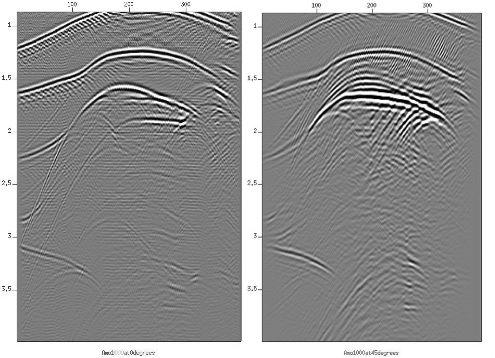
The left hand side of Figure  12 shows a 1000 meter offset slice through an AMO'd volume processed to achieve zero degrees azimuth. The right hand side shows the same line from a similarly processed volume at 45 degrees. Note the considerable differences in reflector position even though the model is the same.

Figure 12: A comparison of zero degree and 45 degree azimuths.

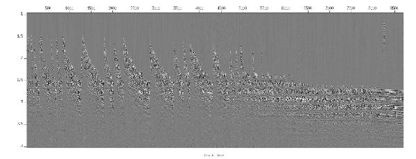
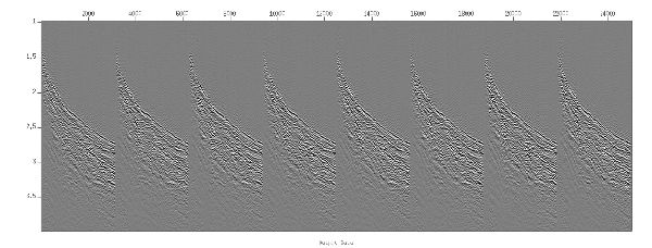
The top half of Figure  13 shows a fixed 15 degree azimuth line selected from a single streamer marine acquisition from offshore Indonesia. Shots with mostly shorter offsets are on the left, while those with mostly longer offsets are on the right. The bottom part of this figure shows a selected set of shots from the 3D AMO processed data set. Note the similarity of these data as well as that all offsets are now present in the common azimuth line.

Figure 13: Real data AMO example