Residual Tomography

Figure 25: Tomographic Geometry

The basic geometry of residual-seismic tomography is explained by Figure  25. We see two source-image-point-receiver raypaths, one in red at a short offset and one in green at a longer offset,. These raypaths represent the migrated location of a reflector at each of these offsets. As each of these rays pass through the cells of the gridded model, it is possible to calculated the total distance traveled from source to receiver for the current migration velocity model. Whether calculated for the red or the green ray, that distance, d, is given by Equation  5, where Δl is the length of the ray in any given grid cell and Δs _mig is the actual migration velocity in that cell.

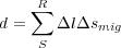(5)

What we are interested in finding is the true velocity, Δs _true. To do this, we calculate Δz for each ray path in the model using Equation  6.

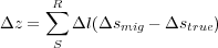(6)

Note that we can measure Δz for each horizon on a CIG, and so we assume we know this value for each and every possible ray. Algebraically, Equation  6 is a matrix equation of the form shown in Equation  7, and it can be solved for Δs.

(7)

Once Δs is known, computation of s _true is straightforward.

In many respects, seismic tomography is very similar to common computer aided tomography (CAT) scans. The primary difference between the two is that CAT scans record purely transmitted energy, while seismic tomography is reflection based. Computer aided tomography reconstructs an image of human tissue by back projecting recorded transmission energy over a straight line. Seismic tomography back projects over a reflection cone. Seismic tomography is also a residual technique. It does not use directly recorded information to estimate the Earth model, and is always based on information extracted from an existing imaging exercise.

Figure  26(a) is an example of residual tomography as it would apply to residual offset dependent depth differences at two line and crossline locations. The figure shows back projected ray bundles indicating changes in velocity as a function of offset from the central line and crossline location.

Residual tomography, as shown in Figure  26(b), is based on the assumption that after a prestack depth migration with velocities that are close to each other, lateral positioning of subsurface events will also be close to correct. This being the case, we can relate differences in depth differences as a function of offset to a residual velocity or slowness increment required to make the arrival on the common image gather flat. To do this, we need to have reasonable estimates of the local dip everywhere in the volume being analyzed. In this figure, the correct or reference dip is measured correctly at the offset determined by the near zero-offset trace, that is, by the green rays. What we measure is the residual depth difference at some other offset (the red rays). If we know the local dip, all this information can be related to a change in velocity that forces the next migration to produce common-image gathers that are much flatter then they were before.

Thus, the input required to perform a residual tomographic inversion is:

• a reasonable migration velocity field
• a picked set of residual depths
• a good set of horizons or some other method for estimating local dip. If horizons are used, there should be as many horizons as possible.

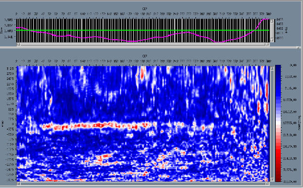
Figure  27 shows what we need to measure to have the proper information to use the method outlined in the previous figures. The right hand side of this figure is a common-image gather after a migration with an incorrect velocity. Note that the curved arrival is close to parabolic or even hyperbolic in shape, but is definitely not flat. The curved green line marks residual depth differences in reference to the shortest arrival. Because the arrival curves down, we know that a velocity above the horizon is too slow to properly correct the horizon at all offsets. Had it curved upward, the velocity in question would have been too fast. Knowing that the velocity is too slow is one thing, but knowing where it is too slow is another thing entirely. What residual tomography does is use redundancy of estimation to determine where to change the velocity to produce flat arrivals. This means that to be effective, tomographic inversion must have sufficient redundancy to do its job. This, in turn, means that we must solve a huge tomographic problem. It also means that a good tomographic solver will have been designed to work from automaticall–picked residuals.

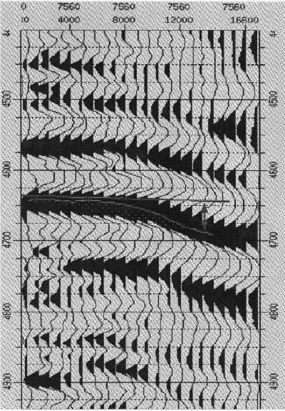
Figure  28 is an example of the use of automatic dip estimation and flattening on a set of CDP's from the SEG AA' data set. Parts (a) and (b) of this figure are illustrative CDP's and their flattened counterparts. Figure  28(c) is the result of stacking the entire suite of CDP's in the line.

Figure  29 is for illustrative purposes only. Residual depths are estimated along horizons. Clearly there is no need for residual tomography at these locations. The colored lines just indicate the depths at which horizons intersect each offset plane.

Figure 29: Residual moveout along a horizon. This is Horizon Based Velocity Analysis or HBVA.

In certain cases, migrating along a predefined horizon (slab migration) reduces computation time and results in faster turnaround time. Figure  30 shows the stack of data migrated along a given 3D surface.

Figure 30: Imaging Along a Slab

Performing percentage-based migration over a horizon can result in horizon-based analysis similar to that shown in Figure  31.

Figure 31: Residual Moveout Along Horizons

Tomographic updating should not be considered to be a technology that solves all velocity update problems. Like its semblance-based counterpart, tomographic accuracy is dependent on the angle range at any given point reflector. As depth increases, this angle range decreases in width until it is too narrow to be of value. Once the angle range reaches a width of less than 10 degrees, tomography is no more useful than traditional semblance-based analysis.

Tomography works best when at any given depth slice, its back projected cones, as displayed in Figure  10, overlap. Again, as depth increases, the degree of overlap decrease and thereby reduces the effectiveness of the tomographic update. Some of these issues can be handled through interpolation or physical and geologic constraints of the type illustrated in Figure  32, but little can be done about the angle range.

Figure 32: Natural Tomographic Constraints

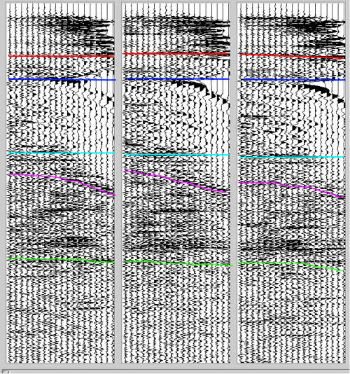
Figure  33 shows the tomographic exercise in graphical form. The left side of Figure  33 shows the horizons which were picked from the initial Dix-based velocity updating. The center graphic of this figure shows the residual depth differences from an automatic picker. The rightmost image in the figure] shows the updated velocity model after the completion of a residual tomographic update. Compare this to the original velocity field in a past slide.

Figure 33: Horizon Based Tomography

Figure  34 contains a side-by-side comparison between a vertical and a tomographic update. The vertical update is on the left and the tomographic update is on the right. Note the velocity inversion (the green on the right hand side of the right figure) and the increased dips roughly in the middle of the right-most figure. This data is over a granitic overthrust in the state of Wyoming in the USA.

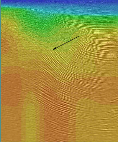
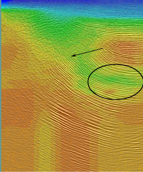
Figure  35 is an idealized flowchart summarizing the concepts and ideas discussed in this part of the course. The first part of this slide embodies what might be called vertical updating. It is only at the bottom thr figure that we actually begin the option to use tomographic updating. Note that tomography is applied only when there is sufficient residual curvature in the output gathers to warrant it. Velocity defined structures, such as salt, are updated through velocity floods. Once the top and base of the anomaly is well defined, residual tomography can be re-applied as needed.

Figure 35: Painless Model Estimation Finalized Workflow

An essential feature of velocity model construction in hard rocks or on land is the increased utilization of wells when available. What is important for this book is the fact that depth migration continues to play its part in the ultimate velocity model definition. In some sense, Figure  36 is more or less identical to the previous soft-model slide. The only real difference is when wells are present is to convert the well information so that it matches seismic times. We can think of this process as check-shot correction, but it is just as easy to do when events at specific times can be matched to specific depths on borehole data. Frequently, velocity anomalies can be resolved in much the same manner as those caused by salt structures in the Gulf of Mexico.

Figure 36: Hard Rock Horizon Based Model Estimation Finalized Workflow