Salt Flood and Body Insert

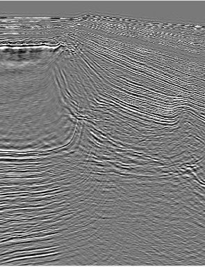
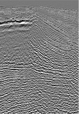
Figure  1 shows several examples of using short-offset salt floods to quickly determine the top and base of complex salt structures. In this case, the offset was limited to 1000 meters and a common azimuth algorithm was used to produce the image.

Each of these snapshots is from a Gulf of Mexico salt structure province and are indicative of the kinds of problems and issues that arise in this setting. Note that interpreting the top and base of salt is quite easy here, but that is not always the case. A major unsolved problem concerns why the salt base is not always visible.

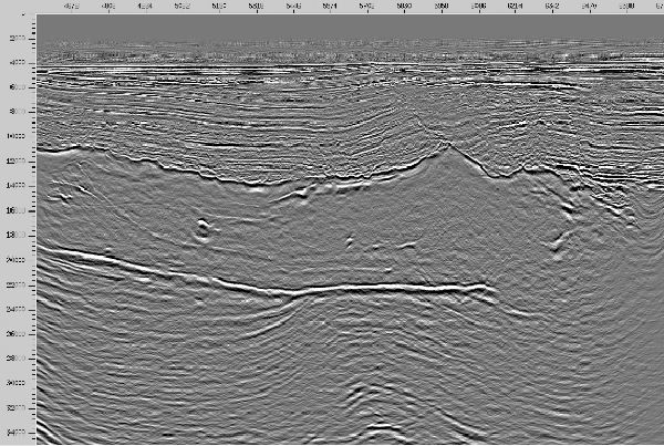
Figure  2 shows a full volume image of a Gulf of Mexico salt structure after completion of detailed MVA and salt body insert. In this image, the salt base and sub-salt sediments are clearly imaged.

Figure 2: Full prestack Kirchhoff volume after salt body insert.

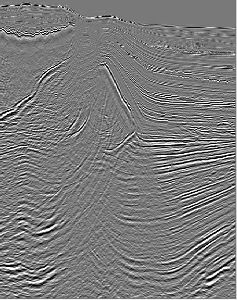
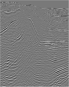
Comparing Figure  3(a) with (b), we observe excessive aliasing of the common azimuth section. This is very likely because the processor failed to properly assess and limit the input frequency content.

The two graphics in Figure  4 show that defining salt body shapes precisely when two salt structures almost overlap can be quite difficult.

Salt structures, like the one in Figure  5, are relatively easy to image with single arrival Kirchhoff migrations. This is mostly due to the rugosity of the top of the salt.

Figure 5: Deep water laminate salt Kirchhoff imaging.