Double Downward Continuation—Common Azimuth Migration

Among the several approaches to prestack imaging, common azimuth migration is one of the fastest. While it may suffer from off-azimuth response problems, it produces usable output at a speed that makes it a viable technique for velocity analysis and velocity model construction.

Figure  18 shows a common azimuth migration. A common azimuth migration parameterizes input data by CDP and offset. Since the data are assumed to have been recorded with one and only one azimuth, the source and receiver locations can be computed from the midpoint (or CDP) and offset. This means that the data are defined by only four parameters: midpoint (2), offset (1), and time, and, as a consequence, are four-dimensional. Normally, data sets with more than one azimuth are really five-dimensional: source(2), receiver(2) and time (1).

Figure 18: Common azimuth downward continuation migration

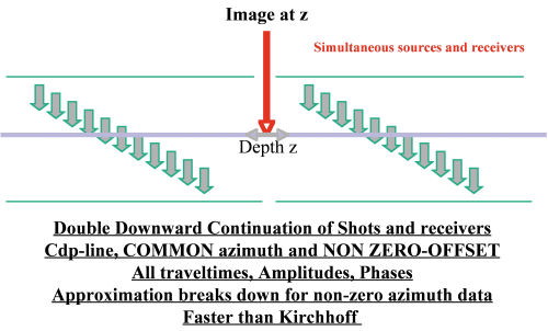
The nice thing about common azimuth data is that they can be continued downward in the same manner as poststack data. Even though the poststack data set has only three-dimensions, the methodology of the two approaches is so similar that we can certainly think of them as being the same.

The disadvantage of the common azimuth approach is that real world data is never acquired in common azimuth form. Moreover, the approximations used to produce the algorithm usually result in a methodology that cannot image steeply dipping events well.

Perhaps the saving grace of this algorithm lies in its speed. For full volume migrations, it has the potential to be the fastest algorithm ever invented for prestack imaging.

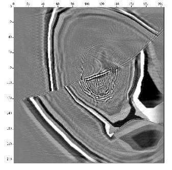
Again, as was the case for poststack data, common azimuth approaches image the data one depth slice at a time. Figure  19 is just an illustration to emphasize that almost all one-way methods image the data one depth or time slice at at time.

Figure 19: Common azimuth depth slice from a migration of the SEG/EAGE C3-NA data set

The nice thing about common azimuth migration is that it reduces the complexity of the input data set by one dimension. Normal 2D data is actually three-dimensional—it is indexed by one space variable for the shot location, one for the receiver, and one for time. In contrast, 3D data is characterized by being five dimensional, where each shot location has at least two surface coordinates, each receiver also has two surface coordinates, and, of course, there is one time dimension. Since shot, m + h= 2, and receiver locations, m h= 2, are a simple function of the midpoint coordinate vector, m, common azimuth data has four dimensions, with two midpoint coordinates, one offset, and time. As a result, downward continuation of data of this type is much simpler that downward continuation of more typical five-dimensional 3D data sets.

However, common azimuth processes are not without problems. For example, the approximations necessary to make the methodology efficient are known to break down at 45 degrees. Furthermore, dip limits can be severe if the implementation does not properly account for different velocities at source and receiver coordinates. Nevertheless, for a large percentage of the subsurface, common azimuth migration is a useful, efficient tool for velocity model construction on a densely-spaced grid.

Aliasing is as much of an issue for common azimuth migration as it is for almost any other type of wave-equation based method. Whether data is recorded at good or bad spatial increments, aliasing must be considered and handled. For example, if it is based on the formulas above, the acquisition dx, dy and desired dz do not support a maximum frequency consistent with the recording parameters, the output spacing can be adjusted so that these frequencies will be imaged without aliasing. Normally, this consideration is not an issue with Kirchhoff-based technologies, since implementations of this type usually handle aliasing correctly without much user consideration. Because it is a recursive process, one-way downward continuation must be performed so that the output spacing precludes any aliasing at every depth step. This is particularly true at the initial downward propagation, but must be maintained until the recorded frequency has dropped below the point where the surface acquisition increments are satisfactory.

In addition to requiring proper spatial increments, common azimuth approaches require input data that is properly sampled in offset. The input offset increment must be chosen to ensure that offset dependent arrivals are not aliased.