Modern Acquisition Geometries

This section describes the physical structure of the commonly used methods of acquiring seismic data over land and water environments.

Cross and Inline Spreads

Modern 3D land acquisition takes many forms. Figure  10(a) shows a typical cross-spread acquisition where shot lines are perpendicular to receiver lines. As the acquisition progresses, the entire pattern is rolled along to cover a large area. This represents true 3D acquisition with large azimuth variation.

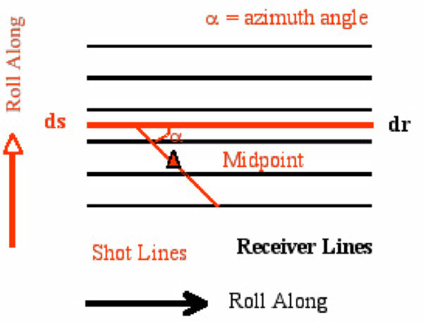
While the data from this kind of acquisition can still be sorted into the usual gathers, it can also be sorted into what are called common azimuth gathers. While this type of shooting produces uniform surface coverage, at least in terms of common midpoints, it usually does not fully satisfy underlying mathematical requirements.

Figure  10(a) shows the geometry of source lines relative to receiver lines for what is called cross-spread acquisition. Figure  10(b) shows acquisition for inline shooting. A grid of receiver lines records the output of sources aligned along source lines. The source lines are separated by ds and the receiver lines are sampled every dr. Both the source lines and receiver grids are rolled-along to achieve uniform surface redundancy. Part (b) shows a typical inline land acquisition geometry. This style is clearly reminiscent of typical 2D split-spread acquisition, and, in fact, the only real difference is that multiple parallel receiver lines recorded each shot response. Like its cross-spread cousin, inline acquisition produces data sets with uniform surface coverage. Because the number of recording lines is small, it usually only produces narrow azimuth data.

As was the case for our split-spread acquisition, each gather from either of the recording geometries in Figure  10 can be migrated independently of any other similar gather. Thus, we can conceive of migrating common azimuth volumes for detailed illumination comparisons. Note that this kind of acquisition produces five dimensional data since there are two coordinates for the source, two coordinates for the receiver, and one coordinate for time. The most important point is that widely spaced lines are good for quick coverage but are bad for spatial sampling.

Sampling will become an issue later when we discuss its impact on high resolution migration algorithms. Although this style of sampling can generate many different azimuths, each azimuth is poorly sampled, meaning that, in some cases, azimuth migration cannot be performed.

CATS, NATS, and WATS

Marine data acquisition has evolved from single cable, single source acquisition to multi-cable multiple source, multiple boat and even ocean bottom (OBC) configurations that can record long offset data in record time. Again, redundant coverage can be sorted into any of the orders discussed in old-fashioned, split-spread shooting.

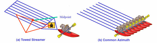
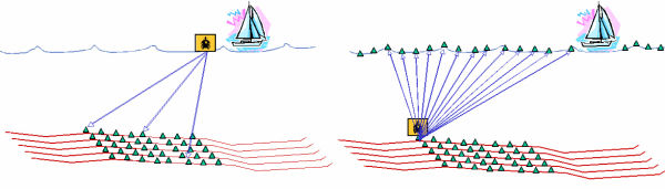
Figures 11(a) and 11(b) show current common azimuth towed streamer (CATS) and narrow azimuth towed streamer (NATS) geometries. There are typically 1 to 20 streamers spanning a cross-spread length from 0 to 2000 or 3000 meters. The geometry on the left has many receiver streamers, while the common azimuth geometry on the right has only one streamer. Although impossible in normal applications, the streamers in the single-ended marine experiment are never really straight. For migration purposes, the cross-spread width should be as large as possible.

Figure 11: Schematic of typical towed multi-streamer marine acquisition.

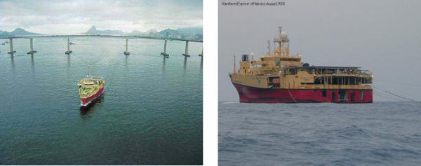
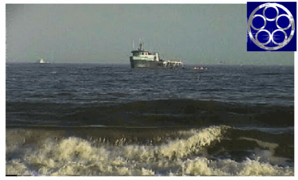
Towed streamers containing a few hundred receivers record data every time the sources, usually air guns just behind boats, like those shown in Figure  12, are fired. Because of boat movement, recording time is usually limited to at most 10 to 15 seconds. Receivers in each streamer data are very finely sampled in each dimension. Cable spacing is rarely more than 100 meters with the number of cables ranging between 1 and 20. The number of traces per shot is large while the shot density per unit area can be relatively low. Although this kind of geometry has been used for many years and has proven to be reasonably good for advanced imaging techniques, it is still somewhat far from what the mathematics and physics demands. An important issue with this approach is cable feathering caused by water currents, which usually means that it is not possible to achieve the precise common azimuth form shown in the right half of Figure  11. Since most of the algorithms we consider must be run on a grid, traces may have to be regularized to that grid to ensure algorithm accuracy and final image quality.

Figure 12: Petroleum Geo-Services (PGS) boats in operation. Note the towed streamers and the triangular shape of the Ramform boats.

Figure  13(a) and (b) show a wide angle towed streamer (WATS) acquisition and composite shot. In WATS schemes, gunboats make multiple passes over the same shot line. One gunboat is placed at the head and to one side of the receiver array and the other is on the same side at the end of the array. The boat towing the receiver array parallels the gunboats, but traverses an every widening path in accordance with each pass of the source boats. Part (a) shows double gunboats recorded by a single eight streamer receiver boat to achieve shot centered receiver arrays. Four or more wider receiver swaths may have to be recorded to produce sufficient data to produce receiver arrays with areal coverage, as indicated by the surface coverage in the composite shot layout in Part (b). The WATS technology may be the first marine acquisition scheme that actually honors the mathematical assumptions underlying seismic imaging algorithms.

The composite shot in Figure  13(b) can contain a huge number of receivers. This figure was constructed based on the assumption that the receiver boat could effectively tow just eight streamers. Utilization of receiver boats towing 16 or more streamers would cut the work load significantly while still producing a composite shot that is much closer to the true mathematical ideal. When 8,000 meter streamers are separated by 100 meters, eight streamer WATS shots have an areal extent of approximately 6,000 meters by 16,000 meters but could certainly cover an area 16,000 meters on a side. As shown by BP, these types of acquisitions do, in fact, produce data sets fully capable of imaging complex subsurface geology.

Vertical Cables (VC)

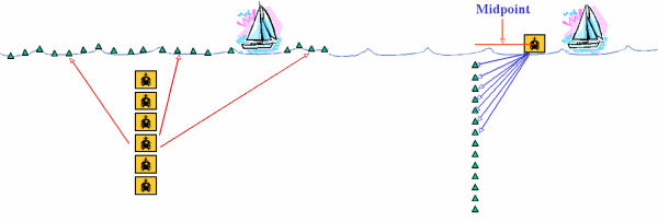
Vertical cables, as shown in Figure  14, are just that. Receivers are actually placed along a vertical cable suspended at a fixed surface location either by sea anchors or by a tether attached to the ocean bottom. Usually source and receiver reciprocity is used to change the acquisition process into an equivalent one where the sources are assumed to be along the cable and the receivers on the surface. While vertical cable acquisition is certainly capable of generating the equivalent of the composite shots of WATS, this particular approach has never achieved its promise, probably because of the inability to keep the cable in a fixed and completely vertical position. Furthermore, processing common receiver gathers as if they were common source gathers is much more computationally efficient than processing common-shot gathers.

Figure 14: Marine Vertical Cable Acquisition.

Ocean Bottom (OBC)

Because gunboats are allowed to shoot in a virtually unlimited set of locations, OBC acquisition can generate areal array shots quite easily. In Figure  15, receivers are laid on the ocean bottom and sources are located on the surface in gun boats like those shown in Figure  16. The receivers on the ocean bottom can be organized into a grid or as a small set of cables similar to those used on the surface. The grid can be positioned on the bottom by a remotely operated vehicle, by a manned submersible, or by simply allowing the cables or receiver unit to sink to the bottom. Wireless communication can be used to accurately locate the entities when in position. Migration of common receiver gathers is normally more computationally efficient than migrating common-shot gathers.

Because the sources are at the surface, the gun boat is free to move in any direction desired. As a result, many azimuths can be recorded during the acquisition session. Data from the receivers can be recorded on the gun boat or on another boat especially designed for recording and processing. If sea-floor cables are used, this acquisition can be very similar to orthogonal shooting on land. The basic difference is that the source boat can move in any desired direction and consequently can generate full azimuth surveys. Usually source-receiver reciprocity is used to view a common-receiver gather as a single shot. When this is done, source spacing and density are extremely important. Because receivers are actually on the ocean bottom, this data usually must be preprocessed almost as if it was land data. Certainly, receiver coupling or lack thereof, and the consequent amplitude differences must be addressed and eliminated or at least suppressed.

Figure 15: Schematic of a typical ocean bottom acquisition.

Figure 16: Fairfield gunboats near shore. OBC acquisition removes many restrictions on where source boats can sail.

Regardless of how they are generated, seismic wavefields are the result of particle motion in the given medium. Figure  17 shows two types of motion: compressional and shear. The red wavefront particles are vibrating tangentially to the wavefront as part of a shear wave. In a medium where velocity varies with angle (that is, an anisotropic medium), there are two orthogonal shear waves. Shear waves do not propagate in a fluid or gas. Particles on the blue wavefront vibrate perpendicular to the wavefront in the ray direction and consequently are part of a compressional wave. Perhaps the best example of a compressional wave is sound in air. Particles in air are compressed and rarified as the wave front progresses. Compressional waves travel in virtually all fluids and solids. Shear waves in solids generally travel at about 60% of the speed of compressional waves. Typical speeds of compressional waves are 330 m/s in air, 1450 m/s in water and about 5000 m/s in granite.

Figure 17: Shear versus Compressional waves

Shear waves are much more difficult to visualize than compressional waves. A good way to think of shear propagation is to consider a deck of cards. It is quite easy to slide the cards in the deck against each other and so generate a wave that propagates through the deck from one end to the other. While this is not necessarily how such waves propagate in the earth, the existence of shear propagation is not in question. Since shear waves cannot propagate in water, it is impossible to record shear waves in the water layer, but this does not mean that marine recordings do not contain shear wave information since all recordings, both land and marine, contain converted wave data. Seismic data from land and OBC data can both contain direct shear reflections, but data recorded in water contains only shear-related compressional waves that are direct conversions from shear to compressional at the water-ocean-bottom interface.

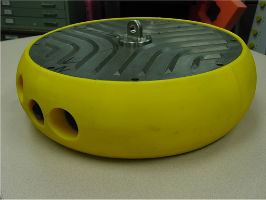
Practical acquisition of OBC data, as shown in Figures 18, 19, and 20 takes several forms. Whether the receivers are cables, as shown in Figure  18, or individual units like those shown in Figures 19 and 20, the primary objective is to place the receivers on the ocean bottom at precisely known locations. However, proper positioning is not always easy to do. In the case of cables, these are usually towed and then dropped. Even with radio sensors, determining their exact ocean bottom position is not always possible. The units in Figures 19 and the more modern version in Figure  20 contain computer systems that can accurately determine position and relay the information back to the recording instruments. In addition, they have sufficient local storage to record several shot responses before they must transmit the data to the primary storage system.

Figure 18: Ocean bottom layout and acquisition. This figure shows the cables and sensors used to acquire data from ocean bottom cables.

Figure 19: This figure shows boxlike ocean bottom receivers being deployed overboard (bottom left and top right) in both deep and shallow marine environments. The top left composite demonstrates that source boats can operate close to shore and platforms.

Figure 20: A modern ocean bottom receiver. Fairfield Industries' latest ocean bottom recorder contains four phones and all the electronics necessary to record source-responses.

The secondary objective of OBC recording is to ensure that each component of the OBC receiver is correctly oriented. Each OBC phone contains a hydrophone, two shear phones, and one accelerometer. The two shear phones must be level and their orientation fixed relative to the rest of the receiver units. Consequently, they are gimbaled and adjustable based on each unit's digital compass. Clearly, OBC acquisition is difficult and potentially expensive.

Regardless of which acquisition method is employed, the net result are data volumes that are truly massive. Figure  21 shows a single time slice through 20,000 square miles of prestack, time-migrated Gulf of Mexico data with an average redundancy of about 90. Simple back of the envelope calculations suggest that the size of this data volume is several hundred terabytes or more. One can easily imagine ocean bottom acquisitions more than four times as large as this one.

Figure 21: This figure shows a time slice from a prestack time migration that essentially covers the Gulf of Mexico Continental shelf. (Image courtesy of Fairfield Industries.)