Migrated Common Image Gathers

There are at least four types of common image gathers that are suited to velocity analysis after migration. You can probably find many more, but for our purposes, the four we explain in this section will suffice.

Common Offset Migrated Velocity Analysis

The best known of these methods is Kirchhoff-based and produces migrated trace ensembles based on migrating common input offset volumes. The advantage of the Kirchhoff method is that we need not output every CIG during the migration process. Indeed, we can focus on local areas, coarse grids, target lines, or just about any form of output to use in the velocity analysis stage. The assumptions of this method are best summarized in Figure  5. It is clear that offset information has been transfered to the output point by simply shifting the source and receiver locations so that the new mid-point is the current image or output location. Figure  6(a) provides the scheme by which such offset gathers are produced.

Figure 5: Migration velocity analysis geometry

Figure  6(a) demonstrates the application of Kirchhoff migration on an offset-by-offset basis. Separating the output data by input offset means that we quite naturally produce input-offset gathers at each surface-defined image point. Such gathers are easily understood by processors used to thinking in stacking velocity analysis terms.

The Kirchhoff method is difficult but not impossible to extend to shot migration approaches. In the case of shot migrations, it is quite easy to produce three gather styles: Angle gathers, shot-profile migrated image gathers, and depth-focusing gathers. All three are based on time-shift, offset-shift, or vertical-shift gathers produced during the prestack migration stage. As we pointed out in the prestack algorithm chapter, these gathers carry information directly related to whether or not the velocity at any give point in the subsurface is accurate or not.

Common Angle Migration Velocity Analysis

Perhaps the best way to understand angle gathers is visualized in Figure  6(b). From a ray-theoretic point of view, we are holding the opening angle (or double the incidence angle) constant and producing output volumes parameterized by the opening angles. Relatively complex mathematics allows us to compute these gathers after the completion of the migration process but before removal of recording redundancy. An advantage of these gather styles is that they can convey considerable information about the kinds of analysis limits we might encounter prior to encountering them.

The production of common angle gathers as shown in Figure  6(b) is essentially the same as the process in (a). The difference is that, instead of holding the input offset constant, the process fixes the subsurface incidence angle to produce common angle gathers. Common angle gathers are certainly worth utilizing, but are somewhat difficult to use and are a bit costly to generate.

Shot Profile Migrated Image Gather Migration Velocity Analysis

Producing image gathers of any useful form from a set of shot-profile images hinges directly on the observation that after migration, the source and receiver are coincident. This fact is independent of migration algorithm—it does not matter whether the input data are migrated offset by offset, shot by shot, or common midpoint by common midpoint. When we migrate offset-by-offset and form common offset gathers based on the original input offset, we are assuming that the image point is directly below the midpoint of imaginary sources and receivers at half the offset distance on either side of the midpoint. Note that this also strongly implies that the migrated data have a fixed and common azimuth. We also expect this to produce precise velocity estimates.

Figure  6(c) represents what we call shot-profile-common-image gathers. A SMIG consists of all shots where the aperture contains a given fixed output image point. The migrated offset in this case is exactly half the distance from the image point to the source location for each trace in the gather. The reason for using half the distance will become clear in subsequent discussions. It is worth noting that SMIGs are not common receiver gathers. Since the fixed point is an output surface image location, they are true image gathers. They can also be three dimensional.

In the case of SMIGs, as depicted in Figure  7(a) and (b), we assume that, after the migration, the image point is directly below a source and receiver, and that it is again separated by a half offset, except that in this instance, the offset is the distance between the image point and the source. It is important to observe that these gathers are not common receiver gathers since surface receiver information is no longer available after migration.

Figure 7: Shot-profile-migrated common image gathers (SMIGs). (a) Graphic explanation shot-profile-migrated common image gathers are formed (b) An example shot-profile-migrated common image gather

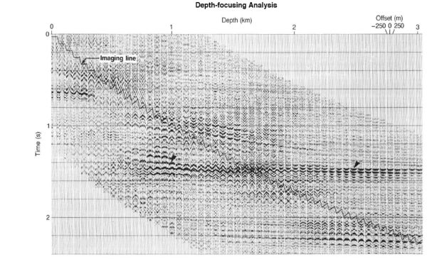
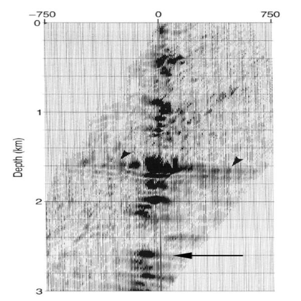
Depth Focusing Migration Velocity Analysis

Depth focusing analysis gathers are essentially the information used to produce angle gathers. They can be formed from either the time-shift or the offset-shift imaging conditions, or even vertical depth-shift imaging conditions described in the section on shot-profile migration.

Figure  8 illustrates the process. Part (a) is a cartoon of forward shot propagation, while part (b) is a similar figure for the backward propagation of the receiver data. By shifting the arrivals vertically, laterally, or temporally, we produce information that can be analyzed to find the maximum energy in the arrival. Figure  9(a) shows gathers produced by a time-shift imaging condition. The horizontal axis in this figure is depth and the vertical axis is time. Part (b) shows the relative depth shift from a fixed position. If the velocities at each depth are correct. the maximum energy arrivals will line up at zero time.