Marmousi Case Study

The original Marmousi data set is somewhat of an enigma. It was designed based on offshore Angola geology and represents a double anticline with the upper anticline sitting virtually directly on top of the lower. The lower structure was prospective but very difficult to image. Neither prestack time migrations or early depth migrations of the day could successfully image the reservoir. Because of this difficulty, Institute Francais de Petrol constructed a model closely resembling the interpreted structure, shot synthetic data over the model and then presented the data to the geophysical community of the day with a challenge to figure out the model from the data alone.

The synthetic data consisted of 240 96 channel shots spaced at 75 meters. The 96 receivers were separated by 25 meters at an offset 200 meters from the shot. Each receiver was the result of summing a more finely sampled array. The wavelet used in this case was neither minimum, maximum, nor zero delay, but produced an effective delay of about 60 ms in the synthesized data. The challenge thus included wavelet processing as well as velocity analysis or inversion and imaging. The goal was to find the velocity model as accurately as possible.

A paper in the 1990's by Sebastian Geoltrain and Roloff Versteeg suggested that Kirchhoff methods alone could never image this structure. While apparently true at the time, as we saw in the chapter on prestack algorithm examples, the real reason this hypothesis made sense was more closely related to the acquisition parameters than to the imaging algorithm.

Our goal here is to see just haw far we can go to produce something close to the actual true velocity. In this sense, we intend to use every available trick in order to achieve our goal

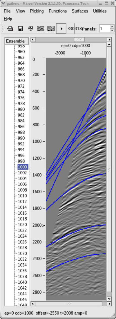
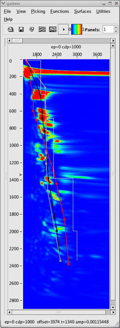
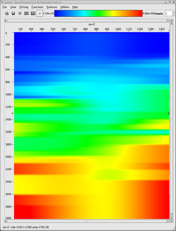
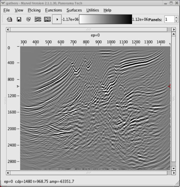
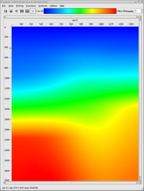
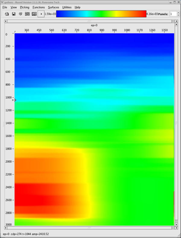
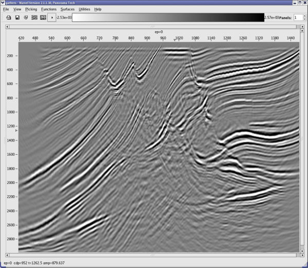
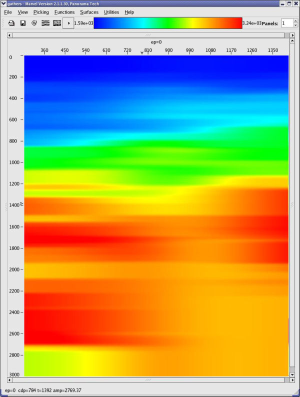
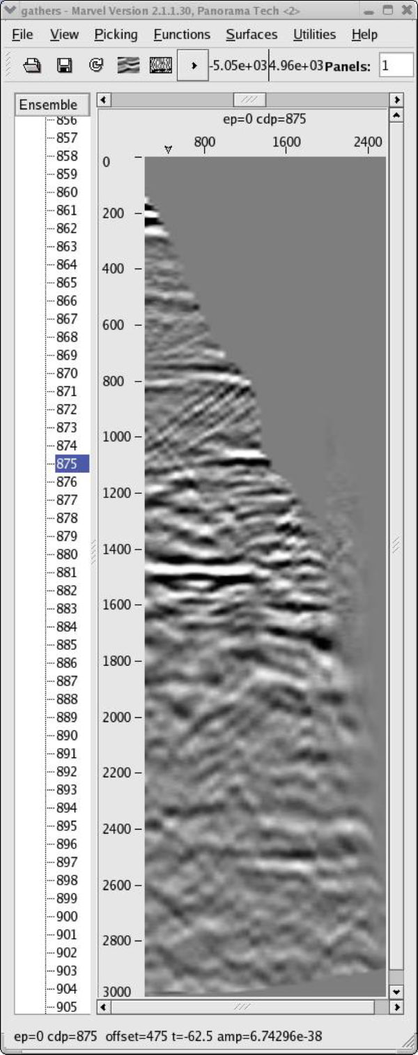
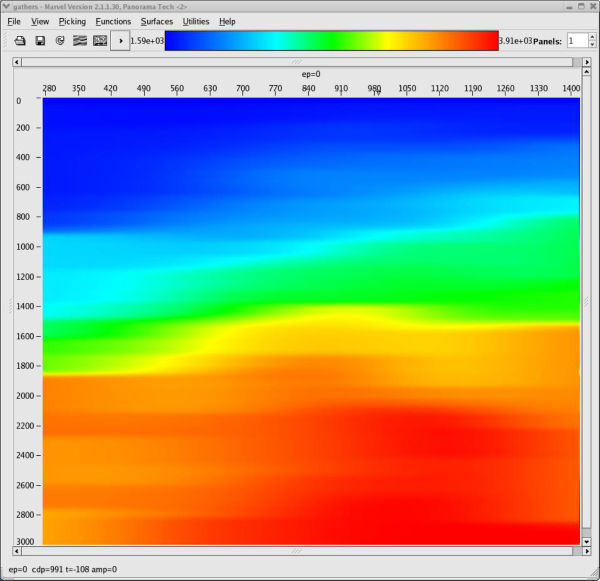
Figure  47 shows typical MVA panels based on the initial stacking velocity analysis shown in Figure  48. Of interest are that

• the stacking velocity model in (a) is extremely smooth
• the Dix depth-interval model in (b) is close to a v ( z )
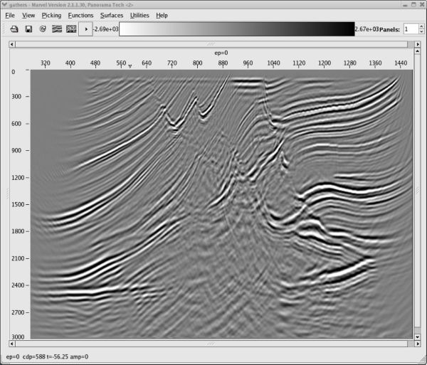
• the image in (c) is essentially what you get doing a PSTM

The smoothness in this case is directly related to the fact that picking was performed on every 100th CDP and that a rather long smoother was applied during the construction of the full model.

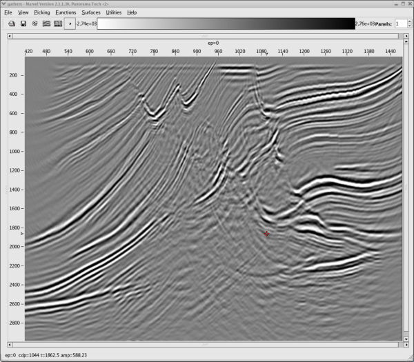
The panels in Figure  47 were used to construct the model in Figure  49. While the changes are not dramatic, it is clear from the depth-interval model in (b) that the geology does not really follow a v ( z ) assumption. Note that the image in (c) is also much more realistic. The only issue in the picking process relates to whether the clear speed up on the left hand side of the model is real or not.

Using the model in Figure  49 as a guide, a new model was constructed from the current prestack data to effect a slow down of the left hand side high velocity zone. The result is shown in Figure  50(b). Note also that the image is now somewhat more realistic, but the gathers are still not completely flat.

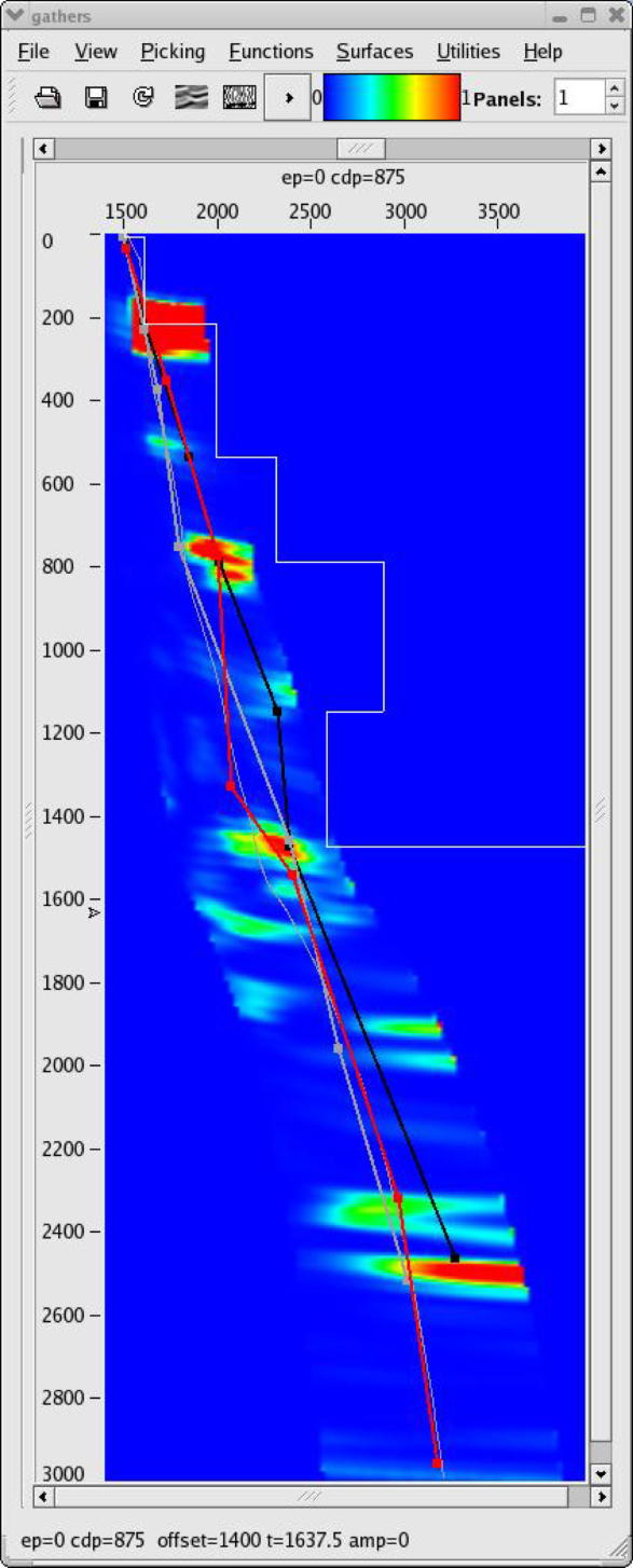
Using the data from the PSDM based on the model in Figure  50, panels like those in Figure  51 were picked and used to produce the model in Figure  52(a) and the migrated image in Figure  52(b). When compared to some of the best images produced in the original Marmousi velocity estimate exercise, this image is not too bad. What is clear is that to improve the answer, several additional iterations will be necessary, but there is absolutely no guarantee that better results will be obtained. In fact, with a nominal maximum offset of just 2600 meters, it is unlikely that velocities below about 1,300 meters per second can be improved much at all.

Is it time to change gears?

Inversion

At this point in any project, we have a velocity model and an image, but we have no idea how accurate the model is. Realistically, we have more velocity models than we know what to do with, and we don't have a clue as to which one is best.

We also have modeling algorithms, so if we believe our model is so good, why don't we test it by shooting data over the model and subtracting the synthetic from the observed data? That is, for each trace in the observed data, generate a synthetic trace, and then create a completely new data set using a trace-by-trace subtraction. If the model is perfect, we get nothing better than completely random noise and we simultaneously validate the model.

But what if we don't get random noise? Is there any way to use the information from the residual to estimate a new velocity model? The answer is yes, of course, and the mathematical recipe is relatively simple. All we have to do is prestack-reverse-time migrate the difference, normalize in the proper manner and add the result back to the current model. Given the new model, we repeat the process of synthetic generation and subtracting. If the new difference is still not zero, we repeat the exercise until the residual can no longer be reduced. This inversion approach was first presented in the geophysical literature by Lailly in 1983, and Tarantola in 1984. When they tested it, it failed rather miserably. We should not let that bother us. The idea looks sound. Maybe they did something wrong, or maybe they just did not have the computer power to test the theory in an optimum manner. Let us do our own test.

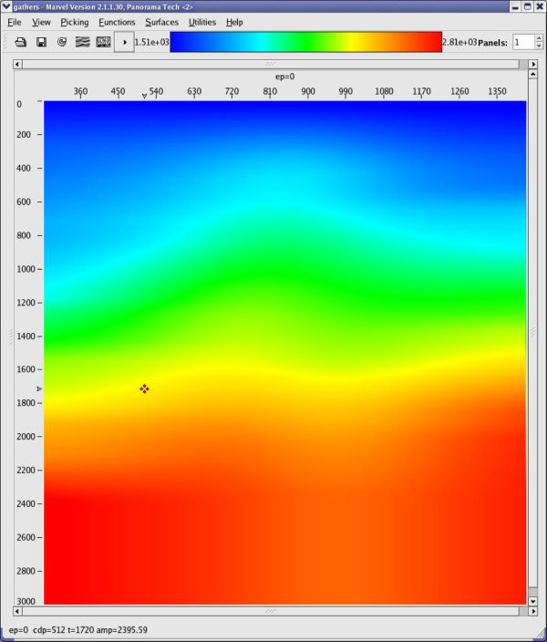
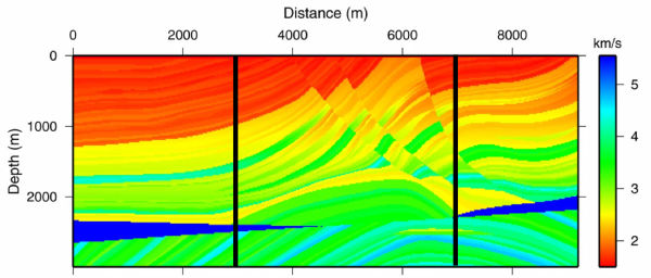
Figure  53 shows the result of testing the theory on synthetic data from the Marmousi model. Starting with the v ( z ) model in (b) of this figure, we synthesized a survey with the same geometry as the data over the model in (a). We then ran the process described above iteratively. The result after 100 iterations is shown in Figure  53(c), and after slightly more than 600 iterations, in (d). Note that the process has worked extremely well. The velocity error in Figure  53(e) is virtually zero, except for those areas outside a offset dependent cone. Note also that the RMS error in (f) has been reduced to a very low level. It is probable that we could have stopped after 300 iterations or so, but we cannot argue with the overall results.

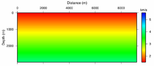
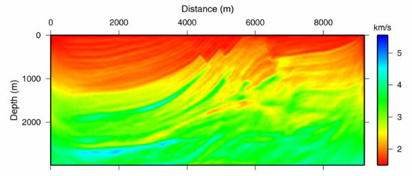
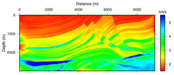
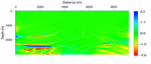
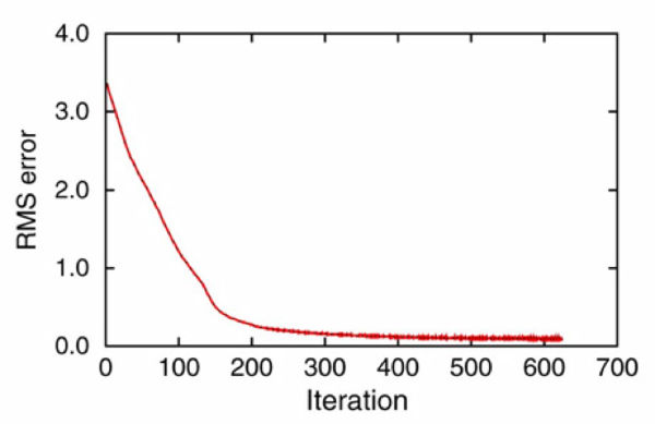
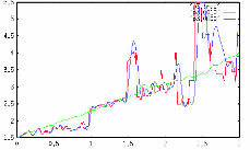
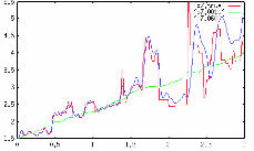
Figure  54 further confirms the high quality of the inversion process. This figure shows logs taken at distances of 3000 and 7000 meters from the left hand side of the model. The green line in this figure shows the initial v ( z ) used to start the process, the red line is the true velocity while the blue line is the inverted velocity after 600+ iterations. Note that down to about 1500 meters, the results are truly outstanding.

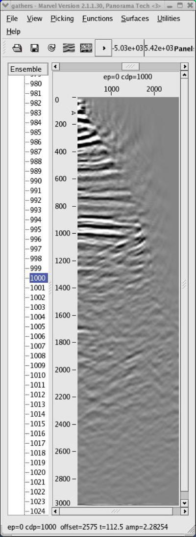
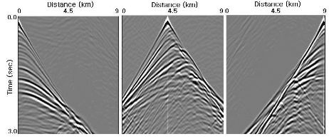
So why did this work now, when it failed so miserably before? Well, to tell the absolute truth, we actually ran the process on extremely low frequency data that we generated over the model in Figure  53(a). These data, shown in Figure  55, extended over the entire length of the model and had a bandwidth that extended from 0.3 Hz to 18.0 Hz. The model was sampled with a very fine grid to minimize dispersion and to ensure that each modeling exercise was as accurate as possible. However, there is no doubt that the real reason this process worked is directly related to the low frequency content of the data.

Figure 55: Marmousi Ultra Low Frequency Synthetic Data