Painless (No Horizons) Velocity Model Construction

Figure  16 shows a typical velocity analysis-velocity model building workflow. This sequence of processes is typically used to convert data-driven-time dependent-stacking velocity estimates into depth-interval or time-RMS velocity volumes. In the painless approach, this process is carried out on flat-lying horizons, and is usually referred to as vertical updating or the Deregowski method. Since we are using a migration algorithm in an attempt to properly position events prior to velocity analysis, local dip information is usually an issue only when the lateral velocity variation is strong.

Figure 16: A no horizon based velocity analysis workflow

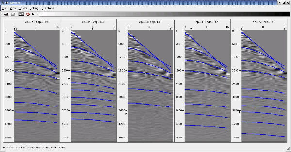
Figure  17 provides one approach to horizon-less velocity model construction. The idea is to directly map Dix intervals to an array of flat horizons at a user-selected fixed depth increment. Note that this Dix conversion is taking place on migrated gathers, and so should produce velocities at locations that are close to the true migrated positions. These intervals are then interpolated to a 3D model along these horizons, where a great variety of interpolation methods can be used. Such interpolation methods range from simple inverse-distance weighting to Gaussian direction oriented balls, or in some cases geostatistical prediction approaches.

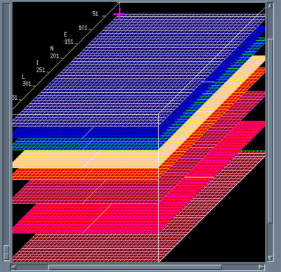
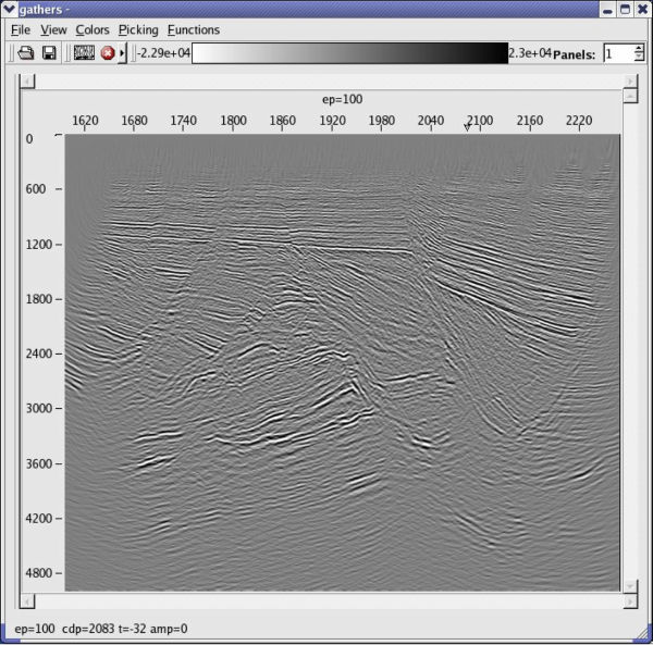
We can summarize the painless approach as follows: Begin with semblance panels like those in Figure  17(b). These can come from stacking velocities or velocity independent time migrations, or from depth migrations using any reasonable velocity field. When picking is complete, interpolation is used to snap Dix-interval velocities to each flat horizon. An example of the result of the interpolation is shown in Figure  17(c). The noticeable bulls eyes are intentional. The interpolation process was modified to ensure that these errors would produce an easy visualization of the location of the spatial velocity grid. In this case, the velocity gradient (blue to red) reflects a significant velocity change across a fault zone. No horizons were used in this process, but the velocity model still reflects local geology. Figure  17(d) shows a final velocity slice after three iterations. Again, the effect of geology is clearly evident in this graphic.

Figure  18(a) shows an initial velocity model generated using a single well hung from the water bottom. The water bottom horizon could come from a high-resolution analysis of the sea floor or from a shallow depth migration with water velocity. Typically, the well information comes from a well within the area extent of the seismic survey. In some cases, the resulting velocity field may be adjusted (sped up or slowed down) to account for depth discrepancies observed in other imaging projects.

As shown in Figure  18(b), MVA on CIGs can be used to painlessly update the initial well-derived velocity model. The model in (b) can then be used to perform a salt flood as shown in part (c). After the top and base of salt is determined, they can be directly inserted into the MVA updated model to obtain the final salt filled model in (d).

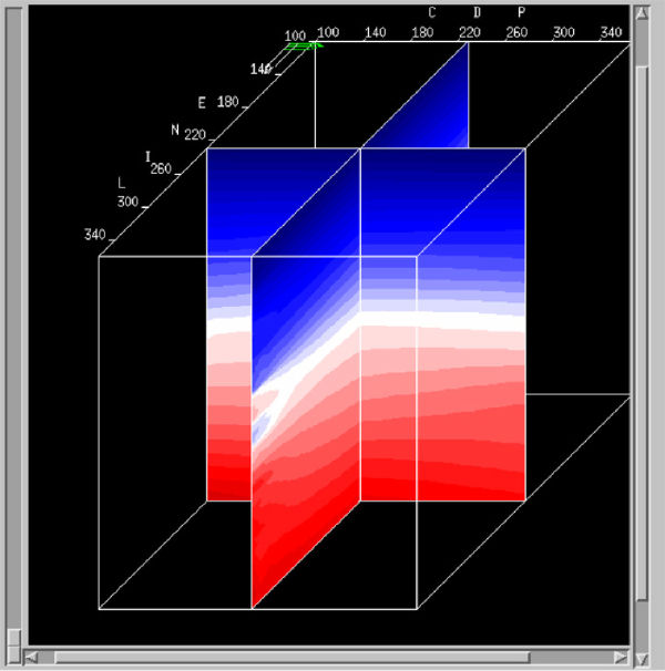
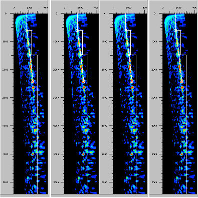
Figure  19(a) is a final image based on the process described in Figure  18. This volume was the result of a common azimuth migration. Note the excellent definition of the top, the base, and the subsalt reflectors. The associated flat image gathers in Figure  19(b) show that the painless approach to Earth model estimation can be quite successful.

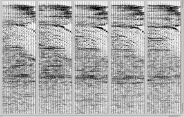
As detailed in Figure  20 (b), prestack time imaging can frequently be done using the painless approach with automatically picked CIGs. When the input data is of high quality, automatic picking can be a useful tool to both assess the need for preprocessing and to quickly provide a useable image.