SEG AA' Case Study

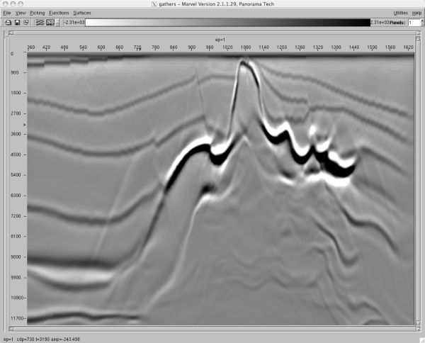
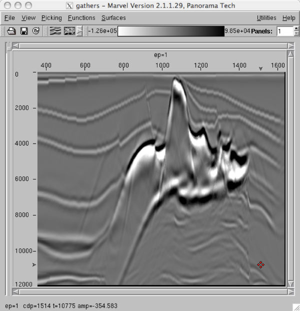
At this point, previous work flows and schemes for estimating depth migration velocity fields may seem a bit daunting. It is probably worth going through the process on a couple of selected synthetic examples where we know what the answer is. Our first example is based on the so-called SEG AA' synthetic. It is really not proper to begin by showing the true velocity model at the start of this exercise, but the interested reader can find that image somewhere below. An automatically stacked version of the input data is shown in Figure  28 above.

Figure 37: SEG AAP coarsely picked background velocity (every 200).

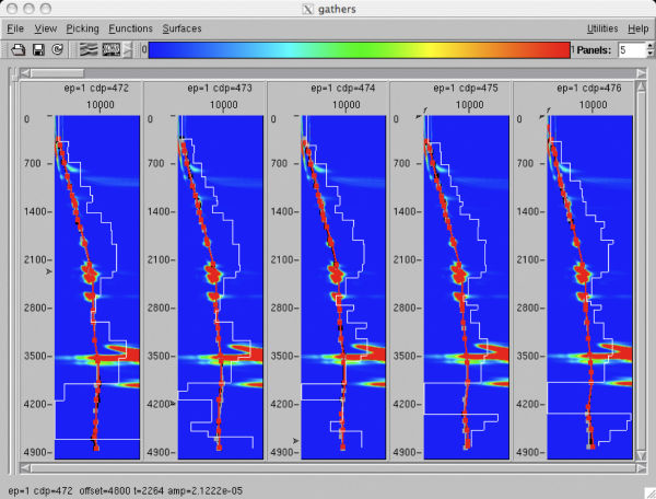
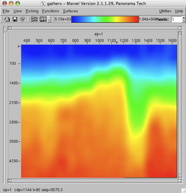
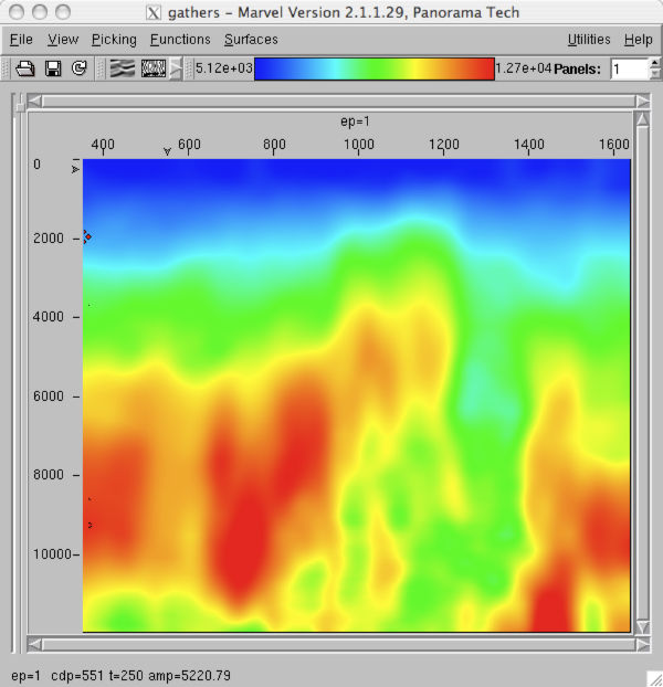
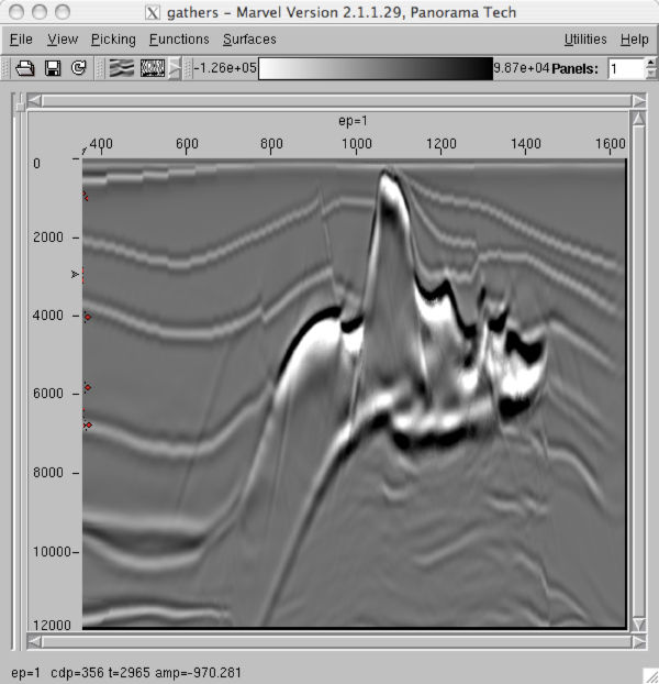
We start the process by first estimating a pre-stack time velocity profile, converting that to depth and then performing a migration of the recorded data. Figure  37 shows a stacking velocity model constructed by picking every 200th CDP from the input data. This is clearly a very coarse model, but its real purpose is to give us a background for automatic picking of the SEG AA' input data. Figure  38(a) shows a selection of automatically picked gathers, while the graphic in (b) illustrates the corresponding semblance panels. The automatic picking used the model in Figure  37 to tightly constrain the picks. Thus, it is not surprising that the stacking velocity model in Figure  39(a) does not vary much from the coarse hand-picked model in Figure  37. The interval velocity model in Figure  39(b) was used to migrate and obtain the image in part (c).

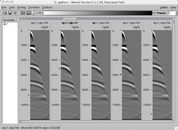
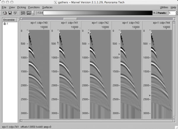
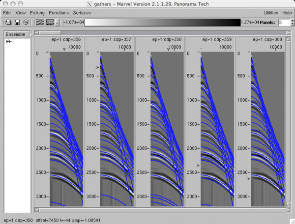
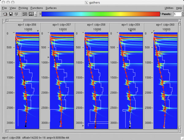
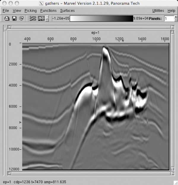
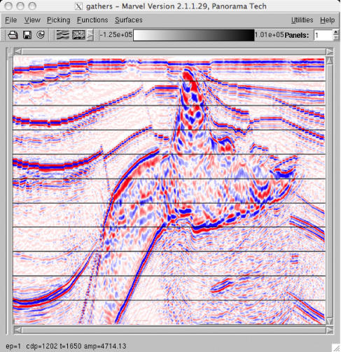
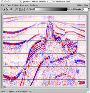
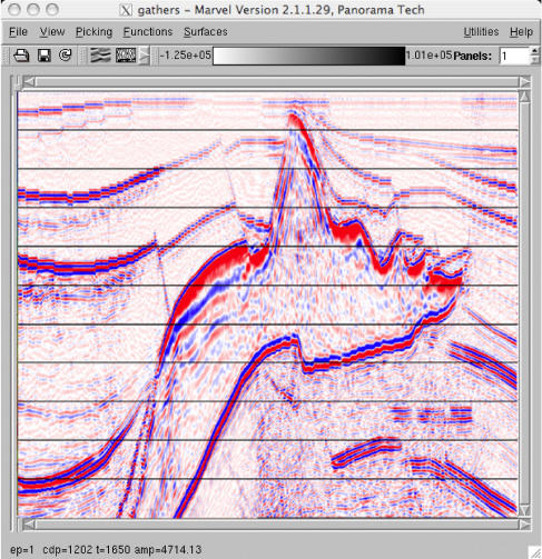
It is clear that we need to repeat this picking process in hopes of improving our image substantially. To this end, we first use the model in Figure  39(b) to time-to-depth convert and apply inverse NMO. Figure  40 illustrates the process. The set of common image gathers (CIG's) in part (a) of this figure show that the initial stacking velocity analysis did not produce a very good model. The gathers are not flat and, in fact, appear to have little or no NMO correction. However, the fully inverse NMO corrected gathers in Figure  40(b) have considerably more moveout, so the migration did improve the flatness of the gathers to some extent. Parts (c) and (d) of Figure  40 are the automatically picked gathers and semblance functions from the inverse NMO corrected time-gathers.

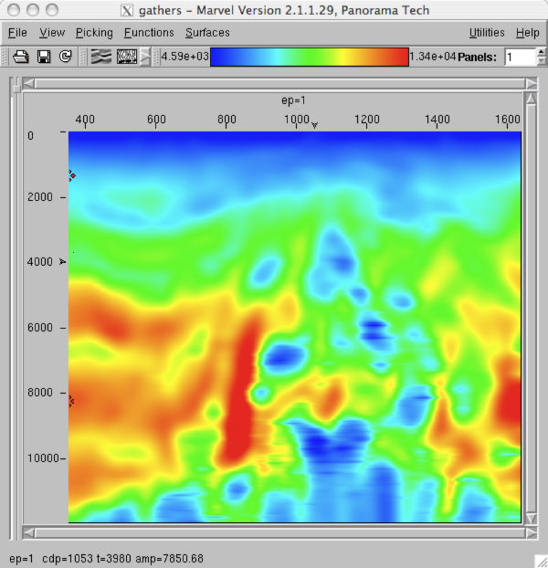
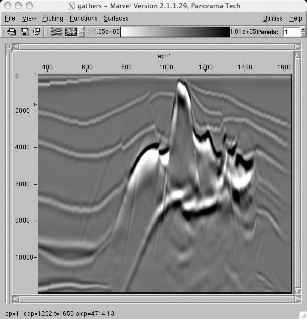
The newly computed velocity model from these picks is displayed in Figure  41(a) and the newly computed image based on this model is shown in part (b). A careful review of the CIG's from this second iteration suggested that it was time to estimate and insert the salt top and base. To this end, the top of salt was picked from the image in Figure  41(b). The salt flood based on the top of salt surface is displayed in Figure  41(c) and the resulting salt flood image is in part (c). The base of salt was defined from the image in Figure  41(c) and the resulting salt body inserted into the model in (a). The result is shown in Figure  41(d). Part (e) is the image based on the model in (d).

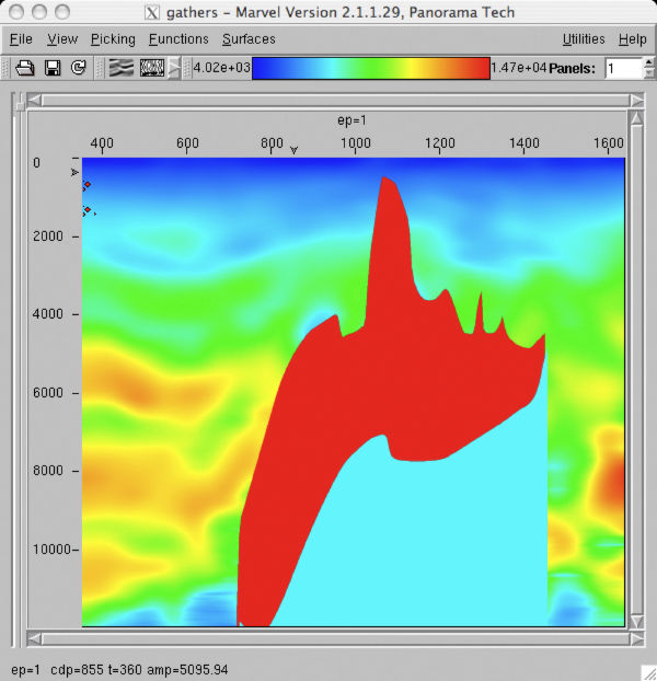
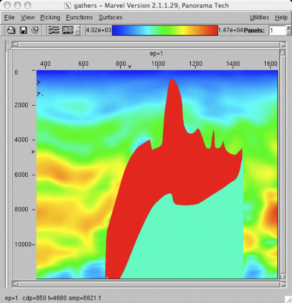
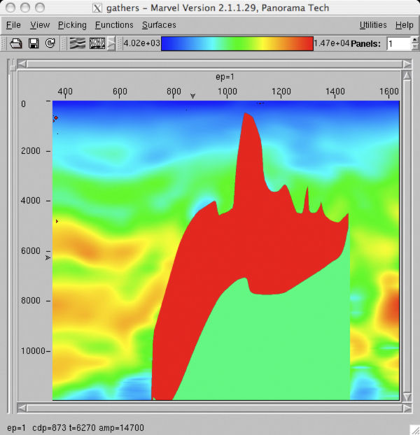
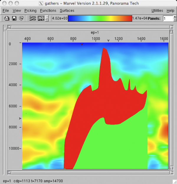
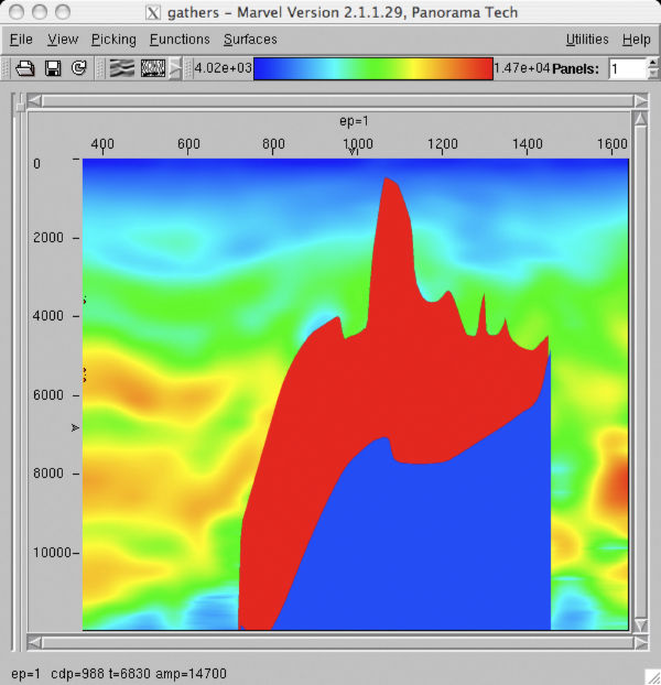
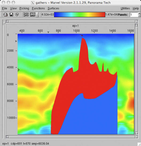
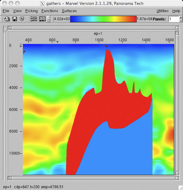
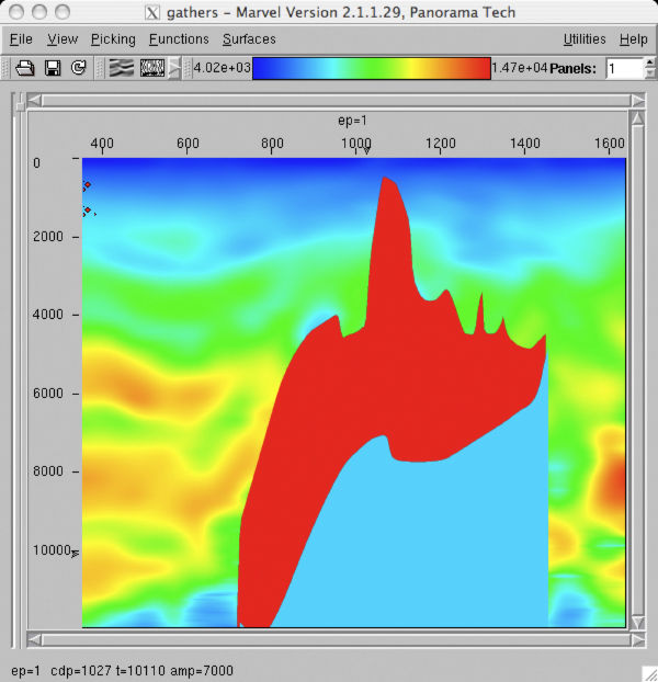
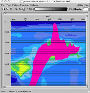
At this point, it is clear that the crude picking-Dix inversion-migration process has produced a reasonable image of what we might call sediments and the salt structure. It is also clear that the image below the salt is not fully geologically sensible. We would think that at this point the way forward would be to keep the salt body in place and complete a very careful re-picking of the CIG's below salt. Unfortunately, the offset range for this example was somewhat limited and almost any velocity below salt produces some kind of image. Thus, it appears that our only option is to perform several additional migrations using models constructed with percentage differences or maybe even constant velocities below the salt. Figure  42 and Figure  43 illustrate this. Figure  42(a) through (k) graphically depict the utilization of what might be called estimated velocities in (a) and (b) through constant velocity increases from 5,000 ft/sec through 7,000 ft/sec in (c) through (l). Similarly Figure  43(a) through (l) depict the utilization of velocities ranging from 7,500 ft/sec through 10,000 ft/sec.

After Tomography

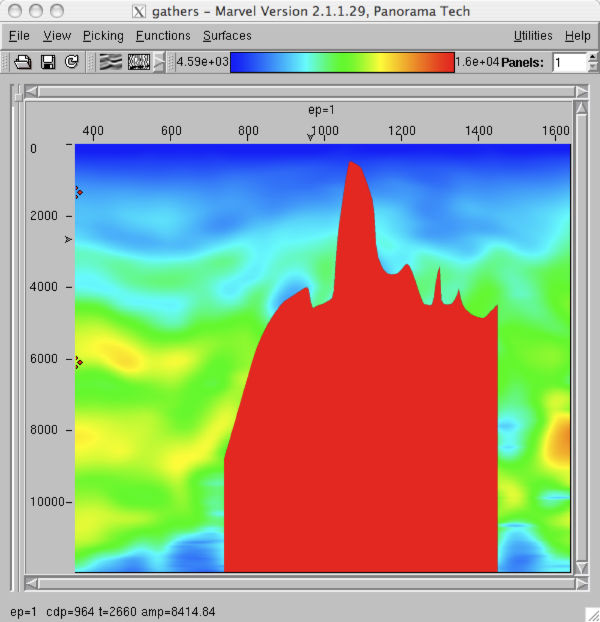
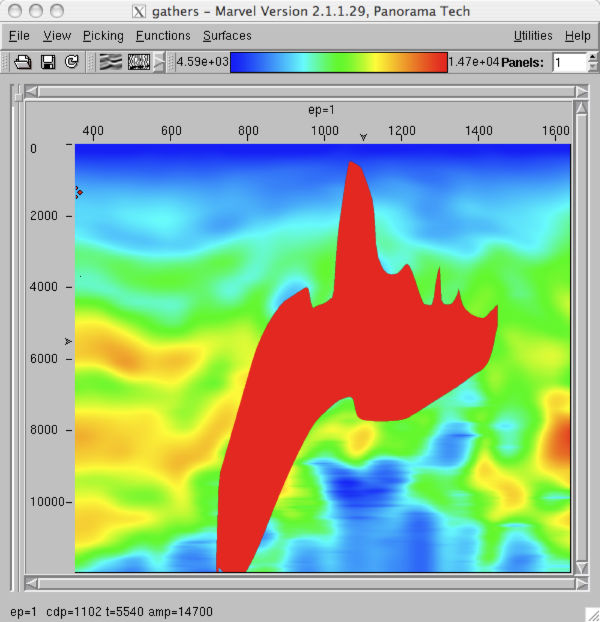
A careful analysis of the migration images in Figure  42 and Figure  43 suggests that the closest correct sub-salt velocity is about 9,000 ft/sec. Based on this assumption, the input data were re-migrated using 9,000 ft/sec below salt and a dip-based-automatic-flattening analysis performed to generated the necessary input for residual tomography. Residual tomography was then applied to generate a new model and the data re-migrated. Figure  44(a) displays the tomographically estimated velocity while (b) shows the true velocity model.

The flatness of the after-tomography gathers is illustrated in Figure  45(a) and (b). The gathers in Figure  45(a) figure are within what might be called sedimentary geology, while those in part (b) fall within the salt regime.

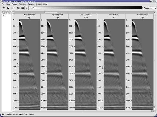
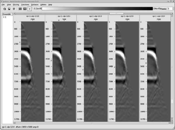
Figure  46 is a full comparison between utilization of the estimated velocity field in Figure  44(a) and the exact velocity field in (b). Note that in every case the one-way algorithm has produced an image that is significantly better than its Kirchhoff counterpart.