The Scalar Wave Equations

From the author's perspective, current state-of-the art practice in digital synthesis of seismic wavefields is usually based on one of four wave equation styles. The simplest style is called the scalar wave equation governing particle motion. Traditionally, this equation involves only compressional style waves and provides a wavefield describing particle motion. Density is assumed constant. The pressure formulation of the wave equation includes density in a form that can be used directly for synthesizing marine style acquisition. The first and second order formulations of what is usually referred to as the stress-strain equations can synthesize both compressional and shear wave data, although at considerable expense in 3D. Thus, in this case the equations govern what can be considered vector propagation. In the simplest case, there are two wavefields, one compressional and one shear. In the more complex case, there are three wavefields, one compressional and two shear. The stress-strain versions are clearly the most interesting because they allow for the most complex anisotropic wavefield propagation.

The 1-D Scalar Wave Equation

In this section we derive a simple one-dimensional version of the so-called scalar wave equation. Wavefields satisfying the various forms of the wave equation are currently our best guess as to how low-frequency-sound energy propagates through the Earth. As we will see, different media require specialized equations, but the basic synthesis or modeling principles remain remarkably similar.

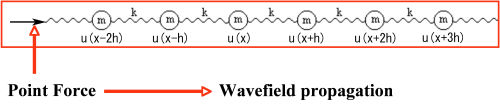
We can gain insight into how particle movement (wave propagation) is governed by considering a simple one-dimensional model. We will start by thinking of the media as a series of discrete particles loosely connected by some form of restraint. Figure  8 shows a series of masses, m, connected together through a series of springs under tension, k.

Figure 8: A simple one-dimensional model. In this case, masses, m, are connected by the equivalent of springs with tension k. A source at one end of the chain creates a wavefield that travels up and down the chain.

If a force is applied at one end of this one-dimensional model, the mass u ( x ) at x reacts with and is acted on by masses u ( x h ) and u ( x + h ). Each such mass accelerates and decelerates as the wavefield generated by the source propagates up and down the model. Note that, although we have suppressed it in the notation, the fact is that u ( x ) = u ( x;t ). In general, we think of each of the masses, u ( x ), as particles that move back and forth as time progresses. What we see is a wave passing up and down the model.

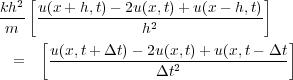
Describing particle movement is accomplished through the use of two fundamental laws of physics, Newton's second law of motion, that is, force is equal to mass times acceleration, and Hooke's Law.

In mathematical form, Newton's law is given in Equation  4, where a is acceleration and m is the particle mass.

(4)

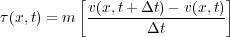
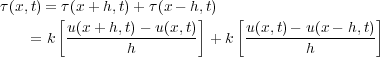
The force caused by acceleration is what you feel when you step on an automobile's accelerator. In the context of Figure  8, acceleration is the rate of change in velocity with respect to time. Thus, for the particle at u ( x ), Newton's second law becomes Equation  5, where τ ( x;t ) is the force per unit area, or stress, at x.

(5)

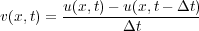
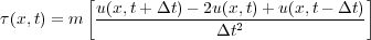
The fact that the velocity is the change in particle position as a function of time yields Equation  6, so Newton's law can be written as Equation  7.

(6)

(7)

For our purposes, Hooke's law can be rephrased as:

Because of the way in which our small particles of mass are arranged, the force ( x;t ) = per unit length is really determined by the action of the particles adjacent to position x. Hooke's law can be stated mathematically as Equation  8 or Equation  9.

If we suppose that there are N masses (particles), each of density ρ, then the total length is L = Nh, the total mass is M = Nm = ρ, and the total stiffness of the array is K = k=N, so we get Equation  10, and, thus, in the limit as h and Δt approach zero, we get Equation  11.

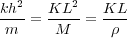(10)

(11)

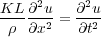
The quantity KL is actually Young's modulus of the medium containing m. It turns out that the quantity v = is the velocity of propagation within the medium, and so we have succeeded in deriving what is normally called the one-dimensional wave equation, Equation  12.

(12)

It is interesting to note that if we combine Equation  7 and Equation  9, and then rearrange the result in the form shown in Equation  13, we obtain an equation that allows us to propagate a wavefield in the one-dimensional medium due to the source s ( x ₀ ;t ) at position x ₀.

If we begin the discussion with both mass, m, and strain, k, as functions of position, x, the velocity, v = v ( x ), of our one-dimensional wave equation will vary as a function of position.

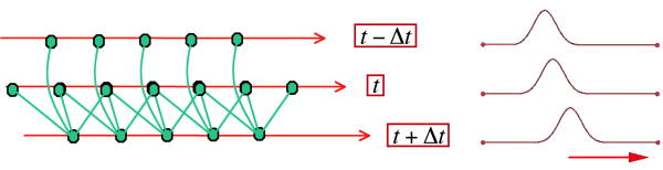
It is clear from Equation  13 that propagation at each time step is achieved through the application of appropriate weights to the wavefields at the two previous time steps. In the case where velocity varies, the weights form a stencil and change for each spatial position. The wavefield at time stamp t + Δt is computed starting at the left most spatial position and continuing to the right.

Figure  9 demonstrates the process. Beginning at the left each spatial output point amplitude is computed as a weighted sum of spatial points from the two previous time steps, that is, t + Δt. The stencil at t is centered around the spatial output point at t + Δt so that waves can propagate in all directions.

Figure 9: Graphical interpretation of a one-dimensional propagator

Scalar Wave Equation in Higher Dimensions

Figure  10 shows a simple model in two dimensions. In this case, masses, m, are connected by the equivalent of springs with tension k. A source placed as a point on the grid creates a wavefield that travels up throughout the grid in all directions.

Figure 10: A simple two-dimensional model.

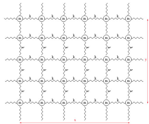
Extending the one dimensional nature of Equation  12 into higher dimensions is not difficult. We need only consider a two-dimensional grid of masses similar to the one-dimensional grid in Figure  8. Our model now has an area A = L _x L _y, instead of length L, a total stiffness of K = , and total mass M = mL _x L _y. Our discrete equation governing wave propagation must accommodate particle motion in both the x and y directions, but, in actuality, this really only involves Equation  9. Thus, if we follow our approach for the one-dimensional discrete equation, Equation  13, exactly, we arrive at Equation  14.

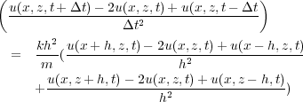
In more compact mathematical notation, the two-dimensional equation in Equation  14 becomes Equation  15.

(15)

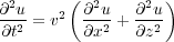
After following the same procedure for a three-dimensional grid, the three-dimensional wave equation becomes Equation  16.

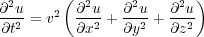(16)

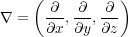
Here, we have derived the mathematical wavefield equations for what is normally called acoustic or pure isotropic modeling. In this case, the velocity was assumed constant, but the difference between a constant velocity and variable velocity derivation is minor. Equation  15 and Equation  16 are referred to as scalar wave equations because there is only one wavefield, not a vector of two or more. Generally, the geophysical convention is to assume that z is the vertical or depth direction, but that is really just a matter of convenience. We could just as easily have used x ₁ for x, x ₂ for y, and x ₃ for z.

Pressure Formulation

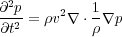
Without going into great detail, we can also derive a pressure formulation of the acoustic wave equation (see Keiiti Aki and Paul G. Richards). This equation takes the form shown in Equation  17.

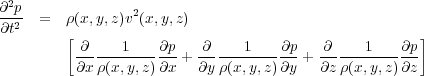
In contrast to the particle motion described by Equation  16, Equation  17 measures pressure changes at any given position. I like to call this the reflection formulation because of the presence of the acoustic impedance term, ρv. This equation can be put in the very compact form of Equation  18, where r is given by Equation  19.

(18)

(19)

Ultimately, we are interested in deriving equations for more complex fully elastic wavefields, including anisotropic. These wavefields require more parameters to describe the multiplicity of wavefields that exist in such media. Before increasing the complexity of the discussion, we will focus on a graphical description of how discrete modeling works, and then turn our attention to algorithms for implementing the actual modeling exercise.