Wavefield and Wave-Motion Hierarchies

In Chapter  8, we noted the possibility of recording elastic as well as acoustic data. Figure  1 shows a simplified diagram of the kinds of waves you might encounter in a typical seismic acquisition experiment.

Figure 1: Wavefield hierarchy

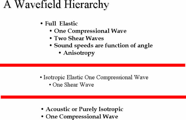
At the top of Figure  1, we see what is probably closest to what happens in the real earth. It is what we should record if we are serious about producing the best possible representation of the subsurface rocks. At the bottom, we see the kinds of waves that most of the migration algorithms of the recent past were designed to handle. This focus on the lowest rung of the ladder was dictated by the lack of sufficient computer power to consider imaging anything other than acoustic waves.

Between these two extremes, we see a wavefield middle ground that was once considered to define a sufficient data set for most, if not all, exploration goals. This has also proven to be false. While it is quite easy to construct middle-ground algorithms based on the technology we have discussed to this point, the possibility of stepping from the bottom rung to the top rung is rapidly making the middle rung obsolete. Moreover, what is important is that zero-offset methods have little or no chance of imaging the complex kinds of waves that occur in the earth. Effective imaging of compressional and shear waves that constantly convert from one to the other can only be contemplated through the use of prestack methods.

Wavefields in almost any medium radiate in all directions. The normal at any given subsurface location to the propagating wave front points in the direction of what we commonly think of as a ray. Since the propagation is normally not constrained with regard to direction, this normal is allowed to point in any direction consistent with the sound speed of the medium. If the normal points upward, we say that this is an upward traveling wave. If it points downward, we call it a downward traveling wave. Clearly, such fields change directions at 45 degrees and become purely horizontal waves at 90 degrees. As we track any given normal or ray, we quickly observe that not only can it travel horizontally but it can also turn up and propagate upward.

Figure  2 shows the kind of wavefields we can model based purely on choice of algorithm. Choosing one of the algorithms defined in Figure  1 means that we inherently assume the propagation characteristics of that particular approach. Unless we happen to choose the algorithm that exactly fits the actual earth propagation, some part of the true wavefield will not be properly imaged. It should be clear that any assumption limiting wavefield directions cannot be correct: It cannot accurately handle amplitudes; it will likely produce artifacts; and it may not be able to image recorded events.

Figure 2: A wave-motion hierarchy.

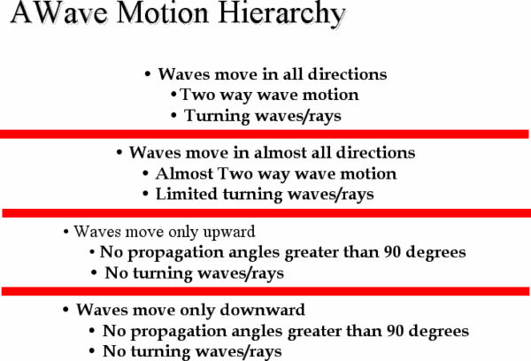
The only good news is that every algorithm in Figure 1 is simply an approximation to the more accurate one at the top. Thus, given results from the bottom level, we should be able to step up to the next level, by simply running the more accurate approach.