Curved Rays

Until this point in time, rays underlying seismic imaging were implicitly assumed to be straight. Allowing the velocities in our Earth model to vary requires that we allow rays to refract or bend. The concept is illustrated in the cartoon of Figure  15. Because light travels at different speeds in air and water, it refracts. Thus, the bowman must shoot below the image of the fish he sees in the water to hit it. When velocities vary significantly, failure to accurately account for reflections along bent rays can cause significant misplacement of subsurface events. This is particularly true in subsalt plays, but is generally true for almost all prospective areas. When this was recognized, migrations began to enter what might be called the depth era. Doing this properly increased the need for a more automated method for producing the stick map images.

Figure 15: Fishing with a bow and arrow

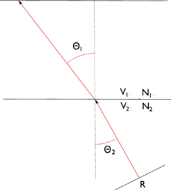
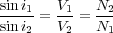
If the bowman is to hit the fish, he must properly account for the way in which light refracts as it passes from the water into the air. Similarly, the seismic program must account for the way sound is refracted when it passes from one layer to another. Both processes, in fact, obey Snell's law, which states that the ratio of the sines of the angles of incidence and refraction is equivalent to the ratio of velocities in the two media, and is also equivalent to the inverse of the ratio of the indices of refraction. For example, when a sound wave is reflected from R in Figure  16 and travels toward the surface, it is transmitted through each layer according to Snell's law. This relationship is stated mathematically in Equation  2.

Figure 16: Illustration of Snell's Law

(2)

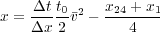
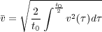
As long as the velocity depends on depth only, curved rays can be incorporated into the migration process by solving the problem layer-for-layer and then integrating. Since depth is unknown beforehand, it is more consistent to sum over vertical time, that is, over the time along a vertical ray. While specific cases can be solved exactly, the general case of arbitrary dependence of velocity on depth requires the two approximations shown Figure  17. As will be seen in later sections, the exact traveltime from surface to reflector is given by an infinite series.

Figure 17: Curved ray corrections

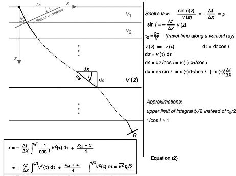
Thus, the upward traveling wave refracts based on its emergence angle, i, in the layer just above it. When it finally reaches the surface with an emergence angle of i ₀, it has traversed the path indicated in Figure  17. The formulas integrating v ( τ ) over τ, provide the necessary estimate of x. The curved ray formula for x is given by Equation  3, where , the well known root-mean-square (RMS) velocity, is given by Equation  4.

(3)

(4)

Equation  3 is important because it tells us how to do an approximate migration when the velocity varies vertically and when rays are allowed to bend or refract. It also provides the mathematical basis for a machine doing the complex migration calculations.

Figure  18 shows how the migration formulas in Figure  17 can be used, in principle, to construct a machine for performing the migration for a given and an average squared velocity given by Equation  5.

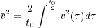(5)

Figure 18: Principle for a analog device for event migration.

For a given , the input values for Δt and Δx are input on the left and the migration distance is read off the sliding cross arm on the right. The different parts of this relation are assigned to corresponding sides of two similar triangles.

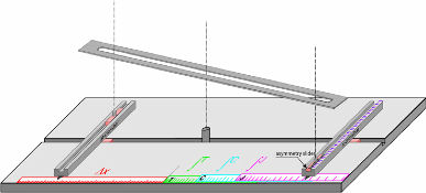
Figure  19 should clarify these comments. Since most reflections were visible on all 24 traces, the Δx setting and the ² setting remains generally constant, at least during the calculation for a single shot record. Since lateral velocity variation was considered to be small, ² also did not change appreciably. What did change was Δt. 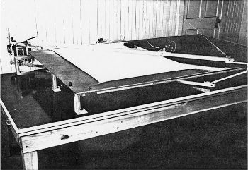This change resulted in a swing of the machine's arm and consequently devices like that in Figure  19 became know as Swing Arms. Figure  20, from A. W. Musgrave's dissertation at the Colorado School of Mines, shows a real migration machine of the type described figuratively in Figure  19.

Figure 19: An early migration machine design.

Figure 20: A. W. Musgrave's version of a swing arm migration machine