Fourier Based Methods

This section discusses the several Fourier-based methods for solving modeling and imaging projects.

FX Finite Difference

The factorization in Equation  106 can also be done in the Fourier or frequency domain by simply rewriting it in the form of Equation  113.

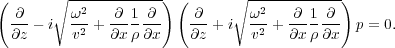(113)

In this case, Equation  110 becomes Equation  114.

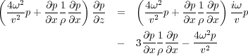
In 3D, Equation  114 becomes Equation  115.

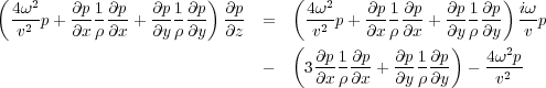
Equation  115 has the generalized form in Equation  116.

(116)

Once again, inversion of A ( ω ) is a necessity. In the frequency domain, this matrix is normally diagonally dominant and usually relatively easy to compute. Note that we are solving this as an equation in z for each ω. We are in effect computing p ( z + Δz ) from p ( z ) so that the A ( ω ) matrix has two dimensions and not three. This further simplifies the issue and makes this method one of the more tractable one way implicit methodologies. Nevertheless, the process is not straightforward and usually requires a splitting approach to make it efficient.

One clear advantage of this approach to one-way forward modeling is the elimination of finite difference approximations in time. In the frequency domain, the partial differentials are simple complex multiplications. Since they are applied across the entire frequency band, the temporal derivatives are as precise as they can be.

Pseudo-Spectral Methods

Pseudo-Spectral methods (D. Kosloff and E. Baysal) are based on the utilization of Fourier transforms in the calculation of spatial derivatives. Again, using the 2D version of Equation  17 as the base, we first apply a central difference scheme in the time direction and then use Fourier transforms to calculate all spatial derivatives. As an example consider the discrete formulation in Equation  117, where L represents the discrete operator containing the spatial derivatives in both x and z.

(117)

To calculate the discrete version of the term , we first Fourier transform in the x-direction on p, multiply by the discrete-spatial wave-number ik _x, and then inverse Fourier transform to get .

This is followed by a repeat of a Fourier-multiply-Fourier inverse step to get .

When the process has been completed along all x-lines, a similar calculation is performed to get .

Working in 3D is just as simple and requires only that we perform one more transform sequence in the y direction.

The great advantage of this process is accuracy. Using the Fourier transform for the spatial derivatives is identical to applying a central difference with the number of coefficients equal to the half length of the discrete transform.

Once we understand that the Fourier transformation converts differentials, into frequency domain multiplications of the form ik _x u ( x ), it is quite natural to want to Fourier transform Equation  17 over all the variables and convert the resulting PDE into a simple algebraic equation. Unfortunately, because the velocity, v ( x;y;z ) and the density ρ ( x;y;z ) are both potentially functions of three independent variables, Fourier transformation would result in a frequency domain convolution, which is not a much simpler algebraic equation.

Constant Velocity FK Modeling

When the velocity v is constant, Fourier transformation over all the variables produces Equation  118 everywhere except at the source.

(118)

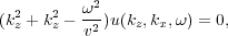
Thus, for k _z and u ( k _z ;k _x ;ω ), we get the equations Equation  119 and Equation  120, respectively.

(119)

(120)

The key point is that we only need to know p ( z = 0 ;x;t ) to determine k _z through a Fourier transform over x and t. Thus, to do modeling we simply define p (0 ;x ₀ ;t ) = s ( x ₀ ;t ), set p (0 ;x;t ) = 0 elsewhere, Fourier transform over x and t, define p ( k _z ;k _x ;ω ) through 119, and then inverse transform to get our one-way modeled data p ( z;x;t ). Whether this represents upward or downward traveling waves is purely dependent on the choice of sign in Equation  119.

Since this method is almost totally dependent on extremely efficient Fourier transforms, you would think that modeling using this method would be very popular. Unfortunately, the equations in this section are valid only when the velocity is constant. As we will see, overcoming this limitation has produced many of the modern one-way algorithms for imaging, but has not resulted in a satisfactory formalism for detailed high resolution modeling. Methods in this section can progress wavefields in one direction or the other, but unlike the two-way methods above do not automatically generated waves traveling at every possible direction.

Phase-Shift Modeling

When the velocity v = v ( z ) is just a function of z alone, and the density ρ is constant, we can Fourier transform over t, x to get Equation  121.

(121)

If we now factor Equation  121 and choose the downward propagating equation as the one of interest, we can write Equation  122.

(122)

If we think of this equation as a first order ordinary differential equation in z, we can immediately write its solution in the form of Equation  123, where k _z has the value in Equation  124.

(123)

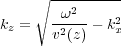(124)

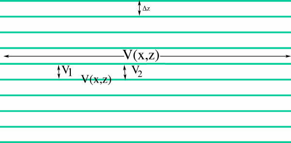
Note that the exponential term in Equation  123 represents a pure phase shift for each frequency ω. The process is visualized quite naturally in Figure  26. Starting at the top for downward propagation and at the bottom for upward propagation, the one-way phase shift method simply shifts the wavefield from one layer to the next in a simple and straightforward manner. To start the modeling process, you initialize the wavefield p ( z = 0 ;x ₀ ;t ) = s ( x ₀ ;t ) at z = 0 with a suitable source, Fourier transform over time and begin downward propagation using Equation  123.

Figure 26: FK domain depth-slice by depth-slice continuation for v ( z ) velocity models. This is called phase shift modeling.

While we recognize that the accuracy of the phase-shift method is highly dependent on the number of terms we use to approximate the series for the exponential, the ultimate accuracy is dependent only on the current computer language approximations for the exponential and the square root. The ultimate limitation of this method, like the pure FK method discussed previously, is the restriction that the velocity vary only in the vertical direction. The frequency slice process specified by Equation  123 has an immediate and more or less obvious extension to 3D.

Phase Shift Plus Interpolation (PSPI) Modeling

When the sound speed, v ( x;z ), varies laterally as well as vertically, the wavefield shifts are no longer uniform. One approach to handling this problem is to first perform a number, n, of pure phase shifts using a uniform set of of velocities lying between the minimum and maximum values of v ( x;z ). Interpolation of the appropriate wavefields at any given x along the common depth slice at z approximates the wavefield corresponding to the true velocity v ( x;z ) at x. Figure  27 illustrates the concept.

Figure 27: PSPI FK domain depth-slice by depth-slice continuation for v ( x;z ) velocity models.

The problem with this approach revolves around the complexities of performing the interpolation. Key questions arise as to whether interpolation in space-time or frequency-space is the more optimum method. Because of the difficulties associated with the need for interpolation, PSPI continuations frequently have difficultly imaging steeply dipping events. As a result, considerable research focused on finding a better approach.

Dual Domain or FKX One-Way Methods

Because of the incredible efficiency of the Fast Fourier transform, it did not take long for several authors to investigate the possibility of avoiding the need for wavefield interpolation by using approximations that split the computations between the FK and FX domains. This required multiple transforms for each up or down shift, but because of the efficiency of the Fourier transform, this was considered worth the extra effort. 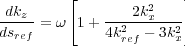The idea underlying this form of the process is again a Taylor series approximation. Let's consider the case where the velocity, v ( x;z ) varies laterally. 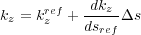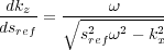The first-term Taylor series expansion of the k _z term in Equation  124 around some fixed reference velocity v _ref = v _ref ( z ) then has the form of Equation  125, where s _ref = is the reference slowness and k _z ^ref = .

(125)

In this case,

(126)

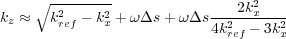
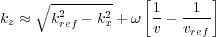
Using the approximation in Equation  107, a little algebraic manipulation yields Equation  127, so that Equation  128, where k _ref ² = .

(127)

(128)

You could, of course, use additional terms of the Taylor series to try to increase the accuracy of the approximation, but, as we will see, the third term in Equation  128 can be quite difficult to implement.

Split-Step

One of the first to utilize Equation  128 was Paul Stoffa at the University of Texas in Austin. He and his colleagues there and at Delft University in Holland simply truncated the series for k _z to Equation  129, and then noted that the first term was just a phase shift in the FK domain while the second is a similar phase-shift in the FX domain.

(129)

Summing over all frequencies produces the image at the current Δz. Fourier transforming back to the FK domain begins the process for the next z + Δz. This method proves to be somewhat inaccurate when compared to good implementations of PSPI, but it is significant in that it requires no interpolation at all. It directly provided a correction in the FX domain after an initial phase shift.

Extended Split Step

The extended phase screen method is probably more accurately referred to as split-step plus interpolation or SSPI. It attempts to increase the overall accuracy of the preceding process by using multiple reference velocities in exactly the same manner as PSPI.

Higher Order FKX Methods

Higher order methods based on Equation  128 must find ways to handle the third term, Equation  130.

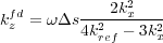(130)

While it might appear that this term can be handled directly by some form of transform between the FK and KX or maybe FX domains, the denominator implies the existence of a singularity and therefore a potentially difficult instability. Two approaches have evolved in an attempt to handle the instability. One is the phase-screen or pseudo-phase screen method of Ru Shan Wu at the University of California at Santa Cruz and the other is the Fourier Finite Difference (FFD) method of D. Ristow and T. Rühl. In fact, both of these methods use what is called an implicit finite difference technique to implement the term stably.

Note that from an implementation point of view, what we do in practice is first form Equation  131, inverse Fourier transform over k _x and form Equation  132, and finally try to compute Equation  133 in some domain or the other.

(131)

(132)

(133)

It should be clear that because the third term contains both spatial and wavenumber terms, this calculation not might be straightforward. The actual trick is to approximate the exponential one more time in the form of Equation  134, substitute back into Equation  133, and clear fractions to get Equation  135.

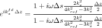(134)

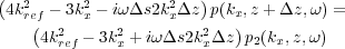
If we now inverse transform back to the FX domain, we see that each k _x ² term becomes a second order partial derivative with respect to x. When these are replaced by central difference approximations, we arrive at a matrix equation of the form in Equation  136, so that Equation  137.

(136)

(137)

What is nice about this method is that the matrix A is usually sparse with a limited number of terms along the diagonal, so in 2D, as described here, inverting the matrix is relatively fast. Moreover, the result is easily stabilized. What is bad about the process is that in 3D the equivalent matrix, A is huge and is quite difficult to invert. The problem is usually solved by a splitting technique similar to that in previous sections. Essentially Equation  135 is solved in the x-direction and then the similar y-direction formula is used to provide a solution in that direction. These methods are alternated as the process proceeds depth-slice by depth-slice until all the data is propagated to the appropriate depth.

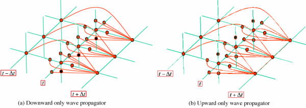
Figure  28 is a simple graphic of how one-way propagators work. Figure  28(a) provides the schema for synthesizing purely downward traveling waves, and part (b) is the corresponding propagator for purely upward traveling waves. While these kinds of propagators limit the type of wave that can be propagated, their significance lies mostly in the fact that they are much more computationally efficient then the full two-way versions shown in previous figures. One-way computations can be performed on a depth-slice by depth-slice basis so there is no need to fill in the value at every previous node before continuing. Moreover, extremely efficient Fourier domain methods can be used to reduce computational complexity even further. As a result, one-way methods have enjoyed great popularity and have been the subject of considerable research.

Figure 28: A one-way propagator. The black dots have been removed from the propagating stencil. Graphic (a) calculates only downward traveling waves while (b) only permits upward traveling waves.