A VTI example
Here we present an example of what one might expect from the analysis process discussed above.
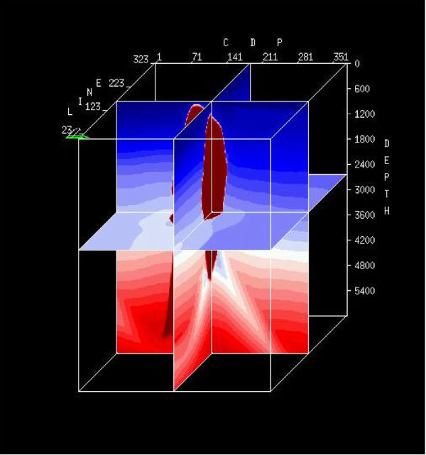
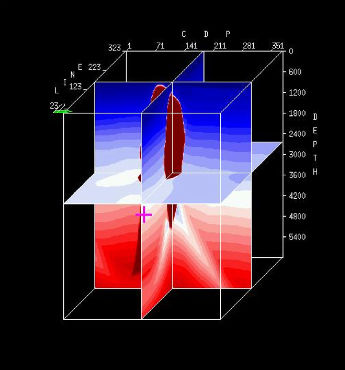
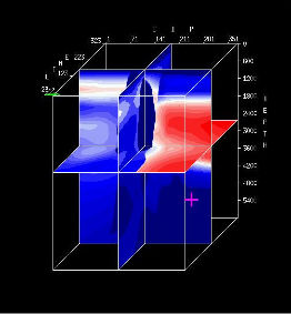
Figure
9 shows a vertical velocity (
v
P
0) field in (a) and a
v
nmo field in (b). Because it is so similar to
the vertical field the horizontal field
v
hor is not shown. What we know from the previous analysis is
that
 | (5) |
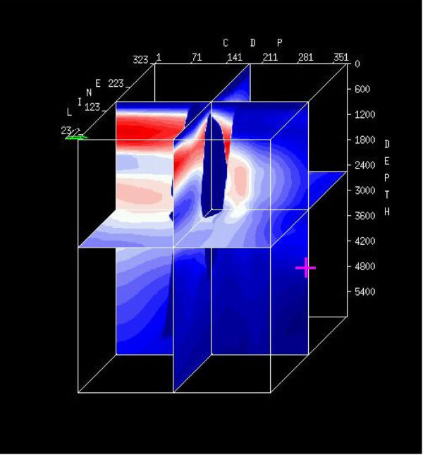
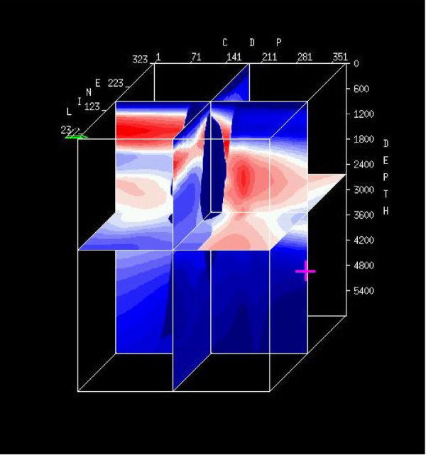
In this case, the
ε volume is shown in Figure
11(b). Given Equation
6, we can easily solve
for
δ, thereby producing a complete three-dimensional volume. The result is shown in
Figure
11(b).
 | (6) |