Stress-Strain Equations

As we know, isotropic elastic models are described by three familiar parameters—density, compressional velocity, and shear velocity. To model elastic wavefields in such three-parameter media, we need to derive a suitable equation or set of equations that describe the wavefield propagation at any given instant. Unfortunately, these three parameters are not the most useful for this purpose. On the other hand, the required parameters are much more directly related to actual rock properties. Moreover, relating the required parameters to more useful quantities is fairly straightforward.

We begin (Equation  8 and Equation  7) by observing that Equation  20 is true, so that Equation  21 is also true. In continuous terms, Equation  21 can be restated as Equation  22.

(20)

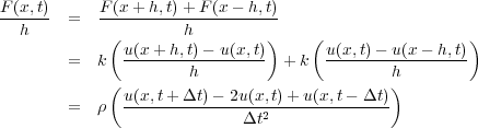
(21)

(22)

Equation  22 is a first order partial-differential equation relating a second order change in time to a first order change in force per unit area. Force per unit area is generally referred to as stress, so our equation relates particle acceleration to stress. In this setting, the stress is one-dimensional and acts along or parallel to the layout of the string. There is also only one compressional wavefield described by this equation. Stepping up to the simple isotropic elastic models described by the three familiar parameters above, means that it is necessary to include one additional wavefield in the mix, namely shear. While including just two wavefields is certainly an option, there isn't any reason not to move up to full anisotropic elasticity by incorporating two shear waves for a total of three wavefields. In three dimensions, Equation  22 takes the form of Equation  23, where i = 1 ; 2 ; 3 and we have arbitrarily chosen to set x = x ₁, y = x ₂, and z = x ₃.

(23)

Clearly, this is a three-dimensional equation with nine stress factors, τ _ij, one for each of the three dimensions and wavefields. To make this into a system of equations governing the three wavefields, we must find a way to relate the stresses, τ _ij to the u _i. As before, Hooke's law comes to the rescue. What it says in this anisotropic case is:

Strain, which measures the deformation (compression, extension, ...) of a solid, is defined in the notation of the previous equation as Equation  24.

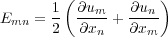(24)

The mathematical expression of Hooke's law then takes the form of Equation  25.

(25)

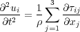
Inserting Equation  25 into Equation  23, we finally get the complex system ( i = 1 ; 2 ; 3) of fully anisotropic equations of motion, Equation  26.

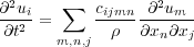(26)

Symmetry

Because equation Equation  26 is three-dimensional, each of the c _ijmn coefficients is actually a three-dimensional volume. Even today's massive supercomputers may not have sufficient memory to handle a problem of this size.

It would not be hard to throw up our hands at this point and give up, but, before we panic too much, we might want to analyze the situation a bit. As it turns out there are at least two things we can do to simplify the situation considerably. First, we can simplify the mathematical notation to put us into a setting where we can make some sense of the parameters, and second, we can reformulate the c _ijmn coefficients in a way that will make a great deal more physical sense.

We are not really interested as much in the math as we are in understanding the kinds of Earth models these c _ijmn coefficients define for us. We need to know how the various velocities of the wavefields that propagate in the medium are defined. We want to see if we can understand how direction changes the speed of propagation, and then see if we can find ways to estimate parameters that can be converted into c _ijmn volumes to both synthesize data and image data we have recorded over fully elastic models.

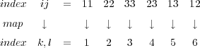
The first simplification to the complexity of Equation  26 is based on the symmetry of stress and strain. Here, the ij indices representing stress can be switched so that c _ijmn = c _jimn. Similarly, the strain based indices can also be switched so that c _ijmn = c _ijnm. Finally, it is also true that c _ijmn = c _mnij. This triple symmetry means that the total number of c _ijmn volumes has been reduced from only 21! Thus, defining the most general model we can imagine requires only 21 independent parameters (volumes), instead of the 81 parameters we would need without symmetry.

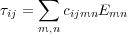
By applying the indexing scheme (known as the Voigt scheme) in Equation  27, we arrive at the 6x6 matrix shown in Equation  28.

(27)

(28)

This matrix completely describes the unique set of 21 coefficients fully defining anisotropic elasticity. In this case, the C matrix is the most complicated form of anisotropy we can encounter. For the interested reader this case is called "triclinic" symmetry and is probably something we will not be able to investigate computationally until computers have advance significantly beyond where they are today. Moreover, we may never be able to measure sufficient data to be able to estimate all of these parameters. Consequently, we will focus on what we consider reasonable today.

Acoustic

In what perhaps is overkill, the C matrix, for a purely acoustic medium, takes the form shown in Equation  29.

(29)

Here, λ is the first of the two so-called "Lame" parameters, which are material properties (proportionality constants) that relate stress to strain. In this case, λ is directly related to the bulk modulus K and the compressional velocity is v _p = = . If we define the actual c _ijmn from the elements of C, plug them back into the fully anisotropic Equation  26, we see that u ₁ = u ₂ = u ₃ = u, and consequently that Equation  26 reduces to Equation  30, which is, of course, the normal three-dimensional scalar wave equation.

(30)

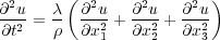
With Equation  30, Equation  23 shows that τ _i;j = 0 ;i ≠ j, _{1 ; 1} = _{2 ; 2} = _{3 ; 3} = , and u ₁ = u ₂ = u ₃ = u, so that it becomes Equation  31.

Equation  31 can also be written in first order form as Equation  32.

Isotropic Elastic

For isotropic elastic models, the C matrix takes the form in Equation  33, where μ is the second of the two Lame parameters.

(33)

In this case, v _p = = . The shear velocity is then v _s = .

It is clear from these relationships, that given density, ρ, compressional velocity, v _p, and shear velocity, v _s, it is quite easy to solve for the coefficients in the C matrix, and then produce the propagation equation for synthesizing isotropic elastic seismic data. It is also clear that modeling with this level of complexity is considerably more computationally intensive than is the case for acoustic models.

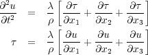
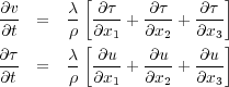
Given the matrix in Equation  33 and then using Equation  23 and Equation  25, we can write Equation  34.

(34)

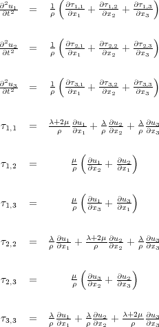
Note that each τ _i;j is expressed in terms of various partial derivatives of the u _i. Back substitution of these expressions into the formulas in Equation  34 for the second order time derivatives allows us to write the elastic particle displacement equation in the form of Equation  35.

(35)

From a practical point of view, Equation  35 says that even in the elastic case we can solve for the vector components of particle displacement u in much the same way that we solve for the non-vector wavefield, u, in a scalar wave equation.

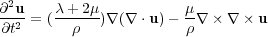
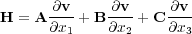
We can also write Equation  34 as a first order vector system. If we take the partial derivatives of the stress-strain terms τ in Equation  34 and let v _i = , we obtain the first order equation for particle velocity, Equation  36.

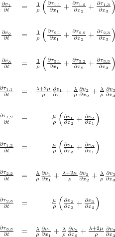(36)

Equation  36 provides a first order system of equations (in time) as opposed a second order system like that in Equation  26. Note that, because of symmetry, we need not write down the terms = , = , or = .

If we define the matrices Equation  37, Equation  38 and Equation  39, we can write Equation  36 in the form of Equation  40, where v = ^T, S ( t ) is a suitable vector source term and Equation  41.

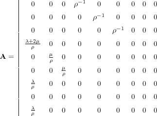(37)

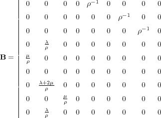(38)

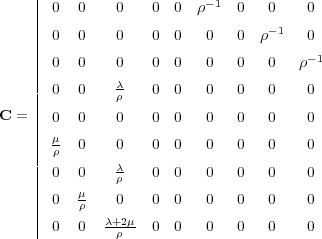(39)

(40)

(41)

Equation  41 is appealing because its a one-dimensional-time-domain differential system whose solution is easily expressed as Equation  42, where v (0) represents the initial conditions.

(42)

When we discuss numerical approximations to this equation, we will find this fact quite useful. It allows us to propagate wavefields one time stamp at a time without having to solve a second order system. It is also easily manipulated to produce a very efficient and accurate forward marching algorithm. Before proceeding in that direction, we continue our discussion of the various types of data we might wish to synthesize.

Vertical Transverse Isotropy (VTI)

The C matrix in Equation  43 defines what has become known as vertical transverse isotropy (VTI).

(43)

Waves propagating in media of this type exhibit a symmetry around the vertical or depth axis, z. Note that the pattern of this matrix is identical to that of the isotropic elastic C matrix. In fact, by setting c ₁₁ = c ₃₃, c ₄₄ = c ₅₅ = μ, and c ₁₃ = λ, the VTI C matrix becomes the isotropic elastic matrix. As we will see, the square roots of the ratios and specify the vertical compressional and shear velocities in the anisotropic medium. It should not be a surprise that the c _ij values in the matrix can be related to intuitive parameters more representative of how we think of the Earth.

We could again follow the development of Equation  36 to produce an equivalent for VTI media, but that is left to the reader. The important thing to notice is that implementation of a discrete version of the resulting first order system will almost certainly follow along the same lines as that for the isotropic elastic case above.

Rock types exhibiting VTI behavior include shales, and thin-bed sequences.

Polar Isotropy

The difference between VTI and polar isotropy is that the symmetry axis is tilted relative to the vertical axis. Early on, this type of anisotropic symmetry was called tilted transversely isotropic (TTI) anisotropy, but in these notes I prefer to use Leon Thomsen's more general term, polar symmetry. Symmetry of this type is easily obtained by simply rotating the tensor c _ijmn of a VTI medium through a fixed angle. The new resulting C matrix produces wavefields that are symmetric around the new symmetry axis. In this case the axis can be relative to any plane through the medium and the propagation is symmetric relative to that plane. Unfortunately, when the symmetry axis is not aligned along the primary axis, neither the C matrix nor the tensor, c _ijmn is particularly simple and generally does not have an easily recognized pattern. This may not be much of an issue since, when the rotation angle is known, it is possible to rotate back forth between VTI and TTI at any time.

Rock types with polar isotropy are identical to those exhibiting VTI, but in this case the symmetry is orthogonal to the dip of the rock.

Orthorhombic Isotropy

Polar anisotropy, including VTI, is always defined by five parametric volumes and the two angles defining the symmetry axis. The C matrix with nine elements in Equation  44 defines orthorhombic anisotropy.

Orthorhombic anisotropy is probably the most realistic anisotropy that we will be able to handle or even use in the forceable future. Again, derivation of a first order system like that in Equation  26 is left your discretion.

Examples of rock types that exhibit orthorhombic symmetry include

• thin-bed sequences or shale with a single set of vertical fractures
• isotropic formation with a single set of vertical, noncircular fractures
• thin-bed sequence, or shale, or a massive isotropic sandstone with orthogonal sets of vertical fractures

Thomsen Parameters

In the mid 1980's, Leon Thomsen's research into anisotropy at AMOCO's Tulsa, Oklahoma research lab lead him to define a collection of parameters that provided a much more intuitive picture of the entries in the C matrix. Thomsen began by defining Equation  45.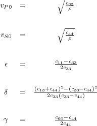

(45)

He then showed that the exact plane wave velocities could be expressed as a function of propagation angle θ using Equation  46, where D 0 is defined by Equation  47.

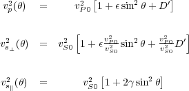(46)

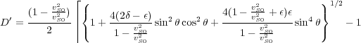(47)

While these formulas have found considerable use for describing anisotropic models and providing propagating equations for synthesis of anisotropic seismic data, the parameters of most importance for this book are the vertical and horizontal velocities. Typically, these velocities are defined from the weak polar anisotropy expressions in Equation  47 with values defined by Equation  49.

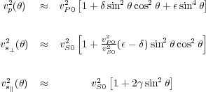(48)

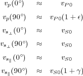(49)

Clearly, ε controls the percentage of anisotropy. It determines the speed of the horizontal velocity relative to the vertical velocity v _{S 0}. What will become apparent as we progress through this book is that δ controls what I will refer to as conversion to depth.

Expressing anisotropic parameters in this manner provides a more natural idea of the parameters defining a polar anisotropic model. While there are many possible variations, such models are defined by four volumes; vertical velocities v _{P 0}, and v _{S 0}, ε, and δ. Equation Equation  26 is then discretized to provide the necessary propagating equation.