Redundant Data

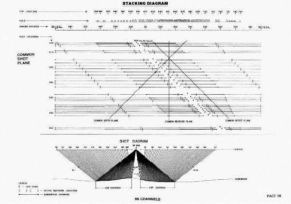
When multi-fold acquisition consisted mostly of 2D data, receivers were laid out on either side of a centrally placed source. Figure  24 shows that this split-spread shooting resulted in redundant data that can be sorted in a variety of ensembles or gathers. In this figure, we see common or fixed-offset, common-receiver, and common-mid-point or common-depth-point gathers. Holding the offset fixed produces sections that, when the offset distance is small, look remarkably like zero-offset profiles. Notice that the term common-depth-point really has very little to do with a subsurface point. It is exactly equivalent to a surface source-receiver midpoint. This is also true of common-offset data, where the offset is measured at the surface. Moreover, these data are completely described when the source and receiver locations for the given trace are known. All other information can be computed from these locations.

Figure 24: Split-spread acquisition geometry.

These data, while usually referred to as 2D, actually have three dimensions: source position, receiver position and time. Alternatively, they can be thought of as having common-midpoint, offset, and time as their coordinate system. However we specify the surface data, the resulting volume is three dimensional.

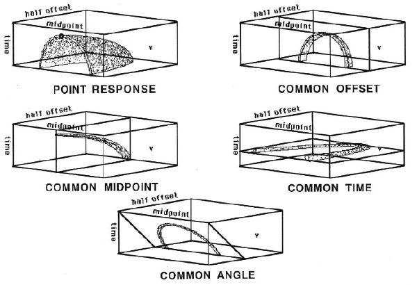
Figure  25 shows the split-spread response of a subsurface containing a single reflection point. At the top left, we see the entire response and then, clockwise, the next four figures show a common-offset slice, a common-time slice, a common-angle slice, and a common-midpoint slice. We will see that there are migration algorithms that allow us to migrate data organized in any of these domains.

Figure 25: Split-spread point response. The response of a single point to split-spread acquisition.

Redundant data have many advantages. In the early days, the major advantage arose because they can be sorted into common-mid-point (CMP) order to produce rough estimates of velocity. Although not completely accurate, these velocity estimates were thought to provide the velocity ² so important in the migration approach discussed above. The accuracy of velocities estimated in this way is a function of many things, but the lateral velocity variation due to reflector dip and the velocity variation due angle of propagation can render such estimates almost useless. Only when the Earth is absolutely flat, and there is no variation of velocity with angle of propagation, can such velocity analysis produce accurate values. Nevertheless, the velocities estimated in this way represented a major step forward in improving the accuracy of migrations. Without these estimates, the production of subsurface images probably would not have arrived as early as it did.

Figure  26 shows how redundant data provides estimates of velocity. The left side of this figure shows a typical common-midpoint gather. The traces all have the same midpoint, and, if the subsurface reflectors are all flat, the hyperbolic curve in red defines the appropriate velocity to use to correct the data to zero offset time, t ₀, and ultimately to produce zero-offset data. Special analog computers were designed and used to estimate ² ( t ₀ ) at as many midpoints as possible. Another analog computer stacked the traces in the CMP and the resulting section was migrated using formulas just like those in the previous paragraphs.

Figure 26: Flat Earth Society processing to zero offset

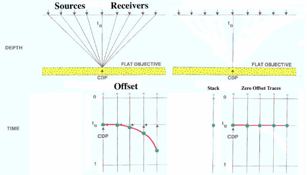
The right hand side of Figure  26 shows the application of a dynamic correction known as normal moveout (NMO) to correct the hyperbolic response to a flat one. Part of the definition of NMO from Wikipedia:

The result of summing the dynamically corrected traces for every CMP is called a stacked section.