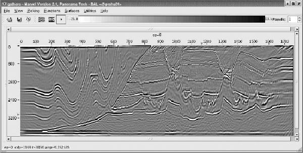
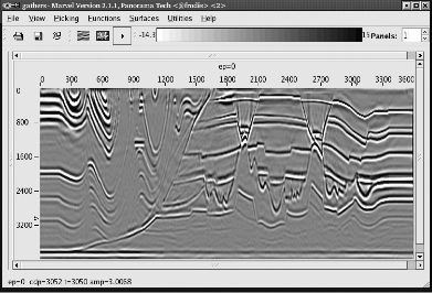
BP 2.5 D Data
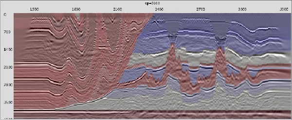
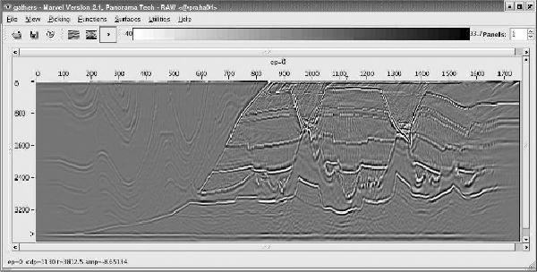
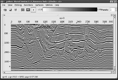
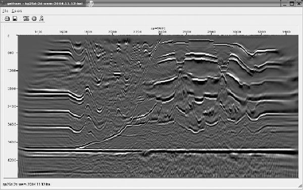
Each graphic in Figure 6 represents application of either a one-way or a two-way method to the original BP 2.5D data set. Parts (a) and (b) show an image of the velocity model overlaid on a one-way image of the raw input data along with the one-way image without the overlay. Parts (c) and (d) show the need to properly account for differences in both illumination and energy spreading losses. Parts (e) and (f) show that use of a well implemented imaging condition can produce dramatic results.
- Introduction
- Seismic Modeling
- History
- Zero Offset Migration Algorithms
- Exploding Reflector Examples
- Prestack Migration
- Prestack Migration Examples
- Common Azimuth on the SEG/EAGE C3-NA Synthetic
- Kirchhoff versus One-Way on a Gulf of Mexico 2D Salt Synthetic
- A North Sea Sill Synthetic
- Marmousi Case Study
- An Imaging Note and the BP 2.5 Dimensional Data
- BP 2.5 D Data
- BP 2004 Salt Structure Data
- SEG AA' Data Set
- Migration from Topography
- The SMAART JV Sigsbee Model
- SMAART JV Pluto Data Set
- SEG/EAGE C3-NA Data Imaging
- Anisotropic Earth Models
- Data Acquisition
- Migration Summary
- Isotropic Velocity Analysis
- Anisotropic Velocity Analysis
- Case Studies
- Course Summary
