Beam and Plane Wave Migrations

Beam and plane wave migrations can be divided into the following cases:

• pure plane wave
• beam stack
• delayed shot
• Gaussian beam

Pure Plane Wave Migration

The migration algorithms in the previous section are all based on downward continuation concepts. Conceptually, each such approach either uses the reversed wavefield as a source term and models the response in reverse, or it uses the reversed wavefield to downward continue the recorded data and produce an image at each depth slice.

The next two algorithms are based on concepts that use surface emergence angles to develop algorithms that produce similar images although they use widely different techniques.

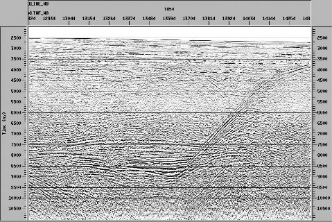
We can also do the decomposition on common-offset sections shown in Figure  25. This is similar to slant stacking a stack. In this case, the section is a synthetic at 1000 meters offset, but for all intents and purposes, it looks just like a stacked section. Note that the short black dip element carries the sum of the information necessary to figure out its final position (the red dip element). A two-point raytracer can figure this out quite easily.

Figure 25: Fixed offset hand migration

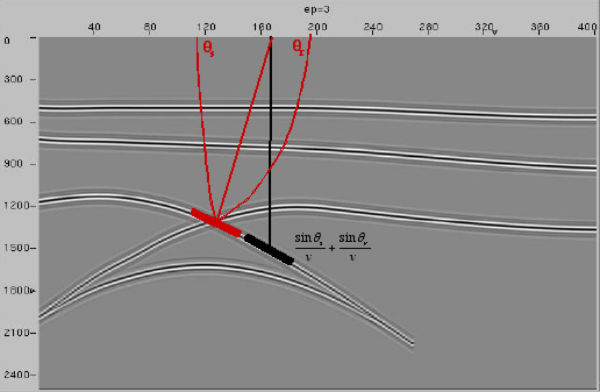
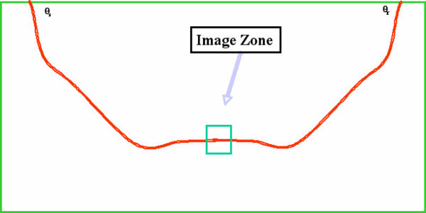
Figure  26 illustrates the process for one of the fastest migrations possible. Given the local dip information from the previous figure, a two-point raytracer gives us the position of the dip element. All we need is a bit of the local wavelet to place at the center of the image zone rectangle.

Figure 26: Ultra fast beam migration

Beam Stack Migration

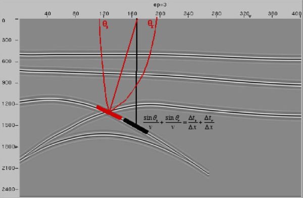
We get a bit more than just the emergence angles when we find the local dip element shown in Figure  27. In this case, the local dip is the sum of the source traveltime gradient and the receiver gradients. Since we know these two values when we calculate the traveltimes, we can construct another beam style migration element through a diffraction stack.

Figure 27: Using local dip estimates

Converting a Kirchhoff method to a beam or slant stack approach requires that we expand traveltime around a central source (or receiver) location in a Taylor series. In two-dimensions, the proper formula is given by Equation  19.

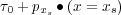(19)

Here, p _{x s} actually turns out to be the derivative (gradient in 3D) of the traveltime with respect to source position; that is,

(20)

Since p _{x s} can be calculated during the raytracing part of the Kirchhoff method, there is little added computational cost. On the other hand, since the entire slant stack bundle replaces many traces in the migration process, Kirchhoff-beam-stack methods can be significantly more efficient than their traditional straight-forward implementations.

Figure 28: Generalized traveltimes and beam-stack Kirchhoff migration (a) Computing traveltimes from centered traveltimes 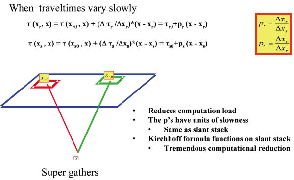(b) Schematic of a traveltime bundle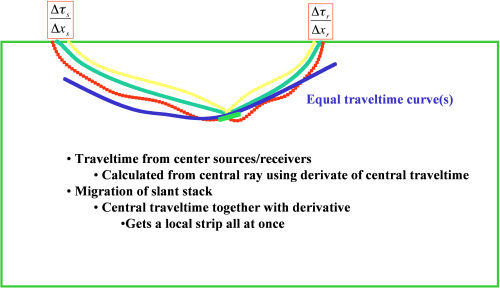

Delayed Shot Migration

Figure  29 illustrates the basic concepts underlying plane-wave or common-emergence angle calculations for source and receiver gather plane wave decomposition. The first step is to decompose the data into plane wave sections. In the case of a synthetic source, we simply decompose the source along the normal to the p value. For receiver gathers, holding p fixed produces a p gather or p-section. Such sections are obtained through a simple slant stack of the data around some central point. To propagate a source, we simply do the propagation along the common angle. To back propagate a receiver decomposition, we simply back-propagate each p. Depending on which algorithm we choose, each common p-section can be migrated individually. After migration, we only need to sum the results to produce a final migrated result.

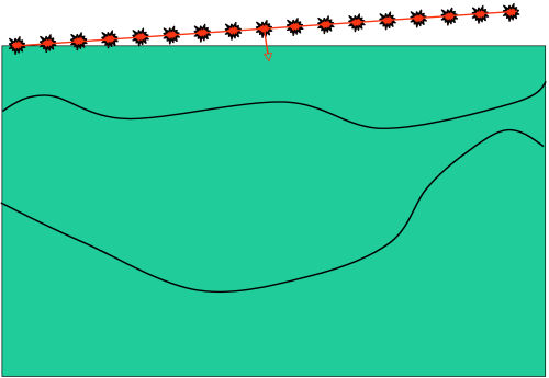
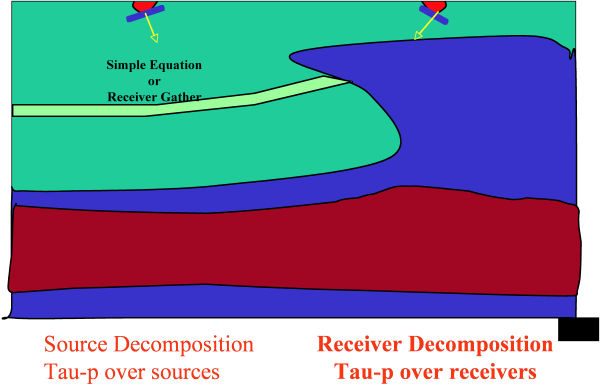
Figure  30 illustrates that each p-value in the slant stack produces a common emergence section that can be migrated in much the same manner as a common-offset stack, or even, conceptually, a zero-offset stack.

Figure 30: A common p section

The utilization of slant-stacked data has many advantages and many draw-backs. An important drawback is the need to use a large number of p-values to adequately cover the entire impulse or operator response. Typically, theory requires us to use hundreds of such values, but most implementations are efficient only if the process uses a few values.

Gaussian Beam Migration

Figure  31(a) shows how a forward propagated shot can be constructed through the use of what are called Gaussian beams. Computation of each such beam requires that we first shoot a central ray. The velocity function, v ( s ), selected along the ray path is then used to propagate source energy forward along this ray. We can use almost any kind of propagator for this process, but usually something like a phase shift is the algorithm of choice. During the back-propagation, energy is allowed to expand from the central ray, and is controlled predominantly by a Gaussian bell-style weight, with the local size depending on the propagation distance and local sound speeds. Because each central ray is defined by its take-off angle, and each such angle is in turn a plane wave direction, we can say that Gaussian beam modeling is really a plane wave modeler.

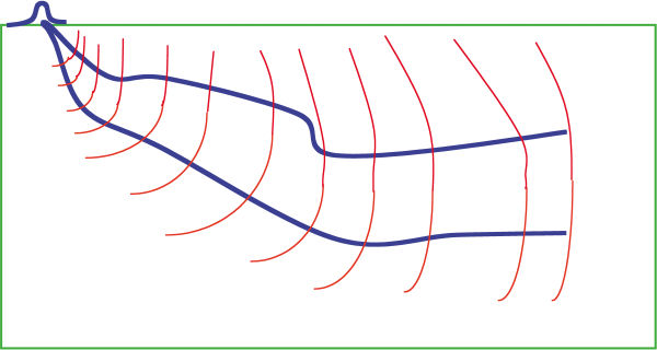
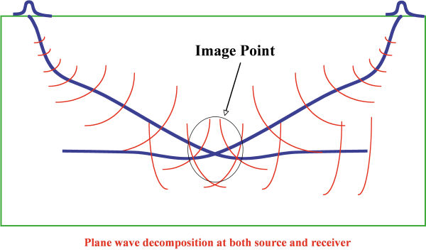
Figure  31(b) shows how to use the concepts discussed in part (a) to construct a Gaussian beam approach to prestack migration. Note that Gaussian weighting is applied to each p-value in the slant stack of a bundle of local traces.

Gaussian beam migration has many positives, including that it does not suffer from the single arrival problems associated with traditional Kirchhoff migrations, and it can be implemented in a manner that correctly handles amplitudes and even multiple arrivals. Consequently, Gaussian beam methodologies tend to produce images that are extremely close to full-wave equation methods. In fact, they are much closer to two-way methods than one-way approximations to the wave equation.