Anisotropic Normal Moveout

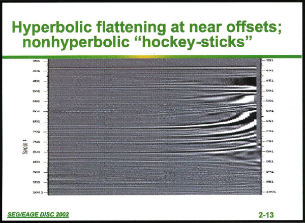
Today we know that the Earth is mostly anisotropic. When we estimate velocities in the isotropic case, we are trading offset information for what we think is vertical velocity. In an anisotropic world this necessarily implies that we are estimating angle dependent sound speeds and as a result we should not expect to produce images that match our wells in any form or fashion. We also should not expect our traditional isotropic velocity analysis to completely flatten common-midpoint gathers. Figure Figure  3 demonstrates what happens when we do. Here we see the so-called hockey sticks so prevalent in anisotropic media. In the past these patterns were usually muted off so as to improve overall image quality. What we really should have done was to try to figure out how to use this information to produce more accurate subsurface images.

Figure 3: After Leon Thomsen DSC 2002. Typical hockey stick character after application of NMO using the usual stacking velocity equation without the anisotripic term.

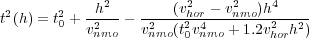
As we saw in the chapter on modeling, the moveout in a VTI medium is specified by the anisotropic normal moveout equation, Equation  26, which has been at least partially empirically corrected in Equation  1.

(1)

Several important observations can be made concerning this equation. The first two terms are identical to the equation we currently use for both time and depth velocity estimation. Thus, we are already familiar with how they work and how we can use them to advantage. Because the difference between v _nmo and v _hor is usually small they are also the dominant terms when the half offset h is relative short.

At first glance this suggests that we can perform an anisotropic velocity analysis as a two step process. The first step ignores v _hor and just estimates v _nmo. Once v _nmo is available a second pass through the data provides estimates for v _hor. As we will see we can also perform a 3D velocity analysis at each vector midpoint for a simultaneous estimate of these important parameters.

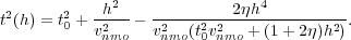
Although known to be somewhat less statistically stable than Equation  1, Equation  2 relates the offset dependent traveltime t ² ( h ) to v _nmo and the so-called η parameter defined by ε and δ as Equation  3.

(2)

(3)

As was the case for Equation  1, once v _nmo has been determined, η can be estimated through a semblance-based process similar to the familiar stacking velocity analysis used to find v _nmo.

These two formulas can also be used in what you might call a simultaneous inversion for either v _nmo and v _hor, or for v _nmo and η. What is different is that the semblance panels are 3D volumes of two of the parameters and time.

Figure  4 is after Tsvankin (2001), where (a) shows an anisotropic arrival curve from a VTI media, and (b) shows the contours of a semblance analysis at 1.0 seconds; in this case, an estimate of v _hor = 2 : 3 and v _nmo = 2 : 0 is quite realistic. Part (c) shows that a value of η : 16 would not be completely inappropriate.

Figure 4: Estimating Vnmo and Vhor

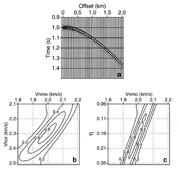
Figure Figure  4 provides a simple glimpse of the NMO based inversion process. Part (a) of this figure shows a single arrival from a reflector embedded in an anisotropic medium. The zero-offset time t ₀ of this reflector is 1 second. In this case, the model NMO velocity is 2 : 0 meters/second, the model horizontal velocity, v _hor, is 2.3 kilometers/second and the η of the model is 0.16. Part (b) of this figure shows a slice at 1 second through a 3D v _nmo v _hor velocity analysis of the data in part (a). Clearly, values of v _nmo = 2 : 0 and v _hor = 2 : 3 kilometers per second are reasonable choices. Part (c) shows the similar panel for v _nmo and η. Since v _nmo is known from part (b) choosing η = 0 : 16 would not be out of line.

Following the process describe above yields three parameters, v _nmo, v _hor. and η. Because η is defined in terms of ε and δ we must find some process which allows us to find either δ, or ε. Once determined we will have achieved the first step is describing a model that describes compressional wave propagation in an anisotropic medium. A quick review of the section on Thomsen parameters reveals that

(4)

Thus, what we need is a process to determine v _{P 0} so we can calculate an estimate of δ algebraically. We measure vertical velocities in a well. Although the measurements are at higher frequencies then seismic sound speeds, these can always be modified as the need arises. This means that we need a process for constructing a vertical well field. Once we have that, we can construct our VTI Earth model from our NMO based estimates, with the exception of γ.