Non-Zero Offsets

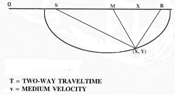
Figure  30 shows the ellipse representing the set of points whose traveltimes from a source at S to a receiver at R are identical. Producing this kind of curve in variable velocity mediums became practical with the advent of digital computers. Migration of fixed-offset data follows the same principles at shown in the zero offset case shown in the bottom image in Figure  27. There is, of course, a corresponding non-zero-offset operator-based approach to migration. Raytracing is used to compute the traveltime from any given source to a reflection point, then from the reflection point back to the receiver on the surface. Operator migration then proceeds in the same manner as it did in Figure  28.

Figure 30: Fixed offset equal-travel-time curves.

It is clear from Figures 27 through 30 that if we wish to use the concepts involved in the most general possible case, we must compute traveltimes from any given source to a potential reflection point and then back to a fixed receiver. Just prior to the advent of digital computers and to some extent beyond that time, efforts were made to do just that. Analog devices were designed to compute these traveltimes in the form of wavefront charts.

The mathematics in Figure  31 was used to compute the wavefront charts in Figure  32. It is not important to understand the mathematics. What is important is that the formulas provide a method for calculating the two-way traveltimes from any point on the surface to any point in the subsurface of a v ( z ) medium and back. Today, the traveltimes originally chosen from wavefront charts are easily and very repetitively computed via raytracing. What is also important is that this approach was known and used in the mid 1950's for performing complex migrated stick figure reconstruction of picked seismic arrivals.

Figure 31: Wavefront chart mathematics

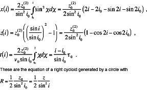
The wave front charts in Figure  32 are based on the mathematics of Figure  31. The charts represent the velocity functions in Equation  7, where n = 0 is constant velocity, n = 1 is standard chart (constant velocity gradient, rays are circles, fronts are spheres), and n = 2 is more realistic, but in the pre-computer days, difficult to generate.

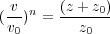(7)

Figure 32: Wavefront charts

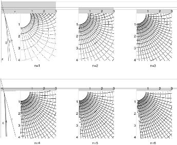
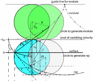
It may not be clear from these figures, but the construction of any given wavefront chart is based on the utilization of circles to generate rays. This should not be too surprising since, for any given constant velocity, the point response is defined by the equation of a circle.

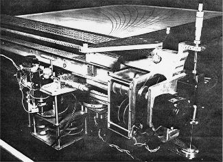
Once the concept, as shown in Figure  33, is understood, it is quite reasonable to construct a mechanical device to both calculate the wavefronts and also produce stick figure images. By the late 1950's and into the early 1960's, machines were constructed to perform migration based on the wavefront charts in Figure  32. Thus, Figure  33 is a geometrical picture of the mechanical basis for a machine such as A. W. Musgrave's wavefront charting machine shown in Figure  34. Note the charts on the surface. This machine is actually an analog device for raytracing. I don't know about you, but this looks like a printing press to me. Unfortunately, no such machine appears to have survived.

Figure 33: The geometric basis for A. W. Musgrave's migration machine

Figure 34: A. W. Musgrave's migration machine

It is important to note that in the real world, because the sources and receivers are at discrete locations, we must consider our measured seismic data to be digital in character. Since modern data is also digital in time, reflection seismic processing today is purely digital. Since the wavenumbers of propagating plane waves carry information about the angle of propagation, this suggests that there will be some issues with regard to the aliasing of dipping subsurface reflectors. The impact of aliasing on our ability to image subsurface events will be discussed in subsequent sections.