Finite Differences

At first glance, finite difference modeling is by far the simplest method to grasp. All that is necessary is to replace the continuous partial derivatives by discrete approximations. The main difficulty arises in producing an accurate approximation to the various derivatives. There are two generally accepted approaches to finding approximations. The first is based purely on some form of fitting algorithm, frequently using polynomials, wherein a set of basis functions with known derivatives approximate the function whose derivative is required. Once the fit is obtained the derivative is defined in terms of the approximating functions.

Polynomial Differences

The easiest approach to finite difference approximation is to simply use a difference quotient in Equation  59 like we did when we derived the full two-way equation.

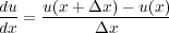(59)

This is what is called a first order forward difference approximation. Similarly, we have the backward difference in the form Equation  60.

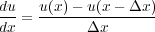(60)

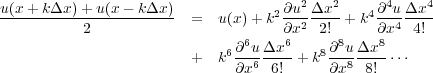
What may not be so clear is that these formulas are the result of approximating u by a straight line between x + Δx and x and between x Δx and x. One of the more popular methods for polynomial approximation is based on the Lagrange polynomial in Equation  61 defined for a sequence of points .

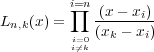(61)

Any function f ( x ) defined that the point sequence can then be approximated by the formula of Equation  62.

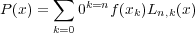(62)

Approximations to the derivatives of f ( x ) can then be approximated through derivatives of the polynomial P . Since P will always be of the form Equation  63, the approximate derivative will always be a weighted sum of the values of f ( x ) at the sequence .

(63)

More accurate approximations can be obtained through the use of other polynomial basis including the Hermite and Chebychev polynomials.

Taylor Series Differences

The Taylor series for u ( x Δx ) in terms of u ( x ) is given in Equation  64.

(64)

If we rearrange this series in the form Equation  65, we immediately recognize that the forward and backward differences are are accurate to Δx. Mathematically, we say that the forward and backward difference are O ( Δx ).

(65)

The Taylor series in Equation  64 can easily form the basis for other more accurate formulas. The most obvious formula arises from the sum of the Taylor series expansions for u ( x + Δx ) u ( x ) and u ( x ) u ( x Δx ). This immediately yields the central difference formula in Equation  66 which is O ( Δx ² ).

(66)

Since we generally think of Δx as being much less than 1 in magnitude, this central difference formula is clearly an improvement over a first-order forward or backward difference.

Second Order Differences

When we summed the formulas for u ( x + Δx ) u ( x ) and u ( x ) u ( x Δx ). we obtained a series that contained odd order derivatives. Accordingly, if we subtract the two formulas, we obtain a series that contains only even order derivatives. This immediately produces O ( Δx ² ) formula for the second derivative with respect to x.

(67)

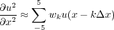
High Order Differences

Extension of the second order central difference formula to higher orders is tedious, but straight forward. For any given k (real or integer), there is Equation  68.

Thus, if we want a fourth order scheme, we take the two terms in Equation  69 and Equation  70, solve the second term for the fourth order partial derivative and substitute the result into the first term to obtain Equation  71.

(69)

(70)

(71)

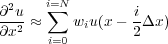
Higher order central difference approximations are obtained by simply adding additional terms to the mix. For example, a 10th order accurate term is obtained by back-substitution in the five equations when k = 1 ; 2 ; 3 ; 4 ; 5. The result is a scheme of the form Equation  72, where the terms are given in Equation  1.

(72)

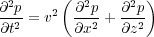
Finite Differences for the Pressure Formulation

We can now formulate a finite difference propagation equation of just about any order we would like. However, it is of interest to reconsider the graphic in Figure  16(b). This figure, based on a simple second-order space-time difference equation shows that to compute any given fixed time stamp, the maximum extent of the stencil is exactly equal to three in each spatial direction and two in time. Thus, to make this process computationally efficient, it is prudent to keep the three t Δt, t and t + Δt volumes in memory at all times.

It is clear from Equation  72 that higher order differences will produce stencils with maximum extent determined by the maximum value of k. Thus, if we chose to use a 10th order scheme for each both space and time, our propagator will be 11 grid nodes wide in each spatial direction and 10 volumes in memory for each of the time stamps t kΔt for k = 5 ; 5. Even with current computational capabilities, holding this many volumes in memory is somewhat impractical. It is natural to try and find a procedure that avoids this memory explosion problem.

Graphical Descriptions

Figure  16(a) demonstrates two-dimensional propagation and Figure  16(b) demonstrates three-dimensional propagation in what is generally called acoustic Earth models. Note that the central difference stencil extends from time t Δt to time t to compute an output point at t + Δt.

Figure 16: Graphical interpretation of (a) 2-D and (b) 3-D propagators.

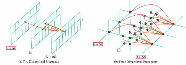
Note that in both cases, the stencil surrounds the ultimate output point to compute the new value. In the 2-D case, the stencil nodes are planar, while the 3-D nodes are volumetric. Thus, the wavefields are allowed to propagate upward, downward, and laterally in all directions as the propagation continues. It also means that we must compute all nodes at step t before we can compute any of the nodes at t + Δt. The examples in the last three figures produce what is called two-way propagation. All waveform styles (for example, refractions, free-surface, and peg-leg multiples) are possible in this setting since these propagators synthesize full waveform data.

Lax-Wendroff Method

Probably the best known "trick", initially published by Peter Lax and Burton Wendroff (see also M.A. Dablain), used the wave equation to find a fourth order accurate difference for that does not increase the overall memory requirement. To understand this trick, consider the case in two dimensions when the velocity is constant and ρ = 1. From earlier efforts, we have Equation  73.

We also know the second order derivative, , in Equation  74.

(74)

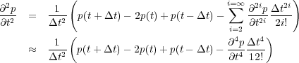
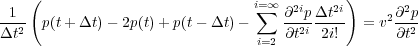
Thus, the fourth order derivative in time is given by Equation  75.

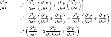
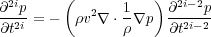
It should be noted that the assumptions of constant density and velocity are not necessary because the Lax-Wendroff scheme generalizes our scheme for finding higher order central difference terms through the recursive formula in Equation  76.

(76)

What we did in the case above was to recognize that higher order time derivatives can be computed from higher order spatial derivatives by applying the spatial side of the original wave equation.

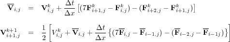
If we now replace the spatial derivatives using formulas like that in Equation  72, we arrive at a fourth order formula for the second partial derivative in time. After calculating all the various weights, replacing partial derivatives with central differences, and solving for p _{i;j;n +1} = p ( i x;j z;n t + t ), we arrive at a discrete central difference formula of general form shown in Equation  77.

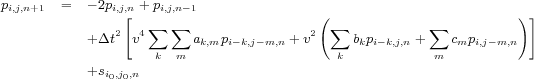
For clarity, Δx ² and Δy ² have been suppressed, and s _{i 0 ;j 0 ;n} represents a source at the location specified by i ₀ and j ₀.

Formulas of this kind are generally called difference equations and provide what is usually called an explicit forward marching algorithm for data synthesis. Schemes of this kind are also called quadrature methods because what they are actually doing is integrating the wave equation to synthesize a response to a given stimulus.

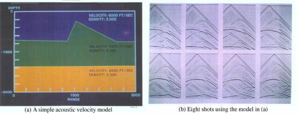
Figure  17 shows a simple pyramid model and data. The finite difference data over this model was synthesized on VAX 11-780 computers in late 1981 and early 1982. At that time, the calculations necessary to compute each shot required on the order of 48 hours. Today, most laptops can compute the entire set of 24 shots in minutes.

Figure 17: A simple pyramid model and data.

Elastic Finite Differences

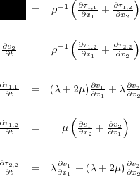
We now turn our attention to discrete simulation of vector elastic data. We can do this using either Equation  35 or Equation  36. Choosing the former leads to a method that is essentially the same the pure explicit finite difference algorithm discussed in the previous. To gain a slightly different perspective, we base our formulation on Equation  36 and again we limit ourselves to the 2D case. In somewhat more familiar notation, Equation  36 becomes Equation  78.

(78)

We note that v ₁ is the horizontal and v ₂ is the vertical velocity of a particle at any given position in space.

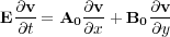
In this case Equation  42 (the evolution equation) becomes Equation  79, where v, A and B are given by Equation  80 and Equation  81, respectively.

(79)

(80)

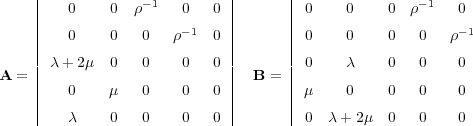(81)

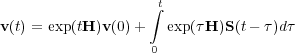
Recall that the solution of this equation has the form of Equation  82.

(82)

Equation  82 is immediately recognizable as a convolution in time. Thus, the progression from initial state to final state is really just a recursive convolution at each time stamp t. The well known series expansion for exp ( x ) provides an immediate approach to providing a discrete evolution equation for the solution vector v ( t ). The resulting scheme is equivalent to the Lax-Wendroff methodology and so will not be discussed further. If you are interested, you are encouraged to work out the mathematical details.

Staggered Grids

What we would like to develop is a finite difference solution to the system in Equation  79. We could, of course, use the higher order difference formulas developed through the use of the system in Equation  70. Several authors (Jean Virieux and A. Lavender) have suggested that somewhat higher accuracy might be achieved through the use of smaller time and space increments. Thus, their idea was to simply rewrite Equation  70 in the form of Equation  83 and Equation  84.

(83)

(84)

This equation, of course, results in a difference formula of the form in Equation  85.

(85)

Note that in Equation  85, the actual derivative is still estimated at a fixed grid point, but the accuracy is based on half the sampling increment.

At first glance it might seem that discrete solution of the system in Equation  78 using formulas based on half derivatives would require significant more storage than using formulas defined at the normal sampling increments. It turns out that this is not the case. We first simplify the notation by defining = so that we can then write v _i;j ^k = v ₁ ( i x;j y;k t ) for any sampling rate, and similarly for w, σ, ξ, and ζ.

A fourth order scheme in space and second order scheme in time to solve Equation  78 can then be expressed as Equation  86.

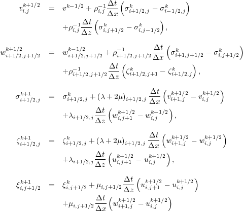
The major difference between this and the usual sampling increment scheme is that the different components of the velocity field are not known at the same node. The actual size of each grid is identical to that of a more traditional equally spaced approach so staggering the grid does not change the overall size of the problem

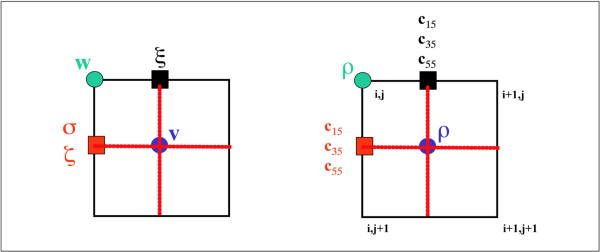
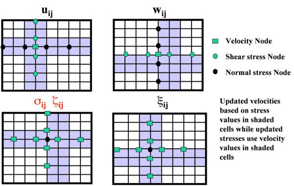
Figure  18 and Figure  19 graphically demonstrate staggered grid propagation. The first of these figures show how the model parameters intermingle with data values at each grid node. The second figure show how each stencil for each of the propagating wavefields is applied. Note that going from one time stamp to the next requires you to cycle through an application of four different stencils.

Figure 18: Distribution of variables and parameters ( ρ;c ij) in a 2D staggered grid mesh.

Figure 19: Staggered grid fnite difference stencils.

It is clear that synthesizing data over elastic models requires significantly more computational resources than when the model is acoustic. Simple isotropic elastic models are described by six volumes, while VTI and full elastic models require seven and eight volumes, respectively. In addition to this increase in storage, the computational load increases by at least one order of magnitude.

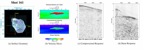
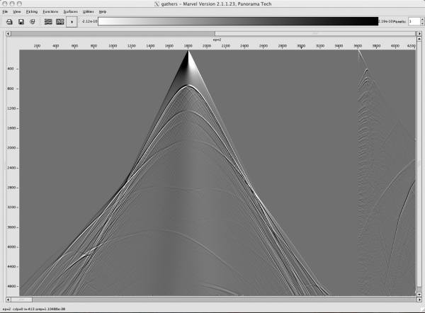
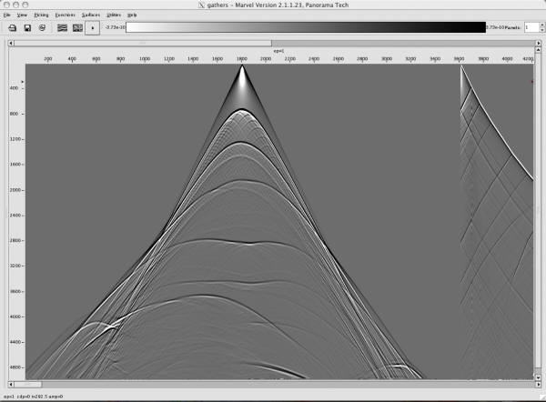
Figure  20 through Figure  24 provide clear examples of simulations over both isotropic elastic and VTI models. Figure  20 illustrates an isotropic elastic version of the SEG/EAGE salt model along with representative in line compressional and shear responses. Figure  21 and Figure  22 show similar images over the Marmousi2 isotropic elastic model. Figure  23 and Figure  24 provide graphics of the full VTI model and VTI shot responses.

Figure 20: Isotropic elastic SEG/EAGE salt model with compressional and shear shot response.

Predictor-Corrector Schemes

Equation  82 can be approximated by a first-order difference to produce the Euler or forward predictor scheme in Equation  87.

(87)

A second order scheme can be obtained by averaging the predicted value with the current value as shown in Equation  88.

(88)

In this case, the x ₁, x ₂, and x ₃ differentials are replaced with suitable central differences, and Equation  88 is used as a predictor-corrector scheme of second order.

Splitting

It is possible to rewrite Equation  79 in the form Equation  89, where A ₀, B ₀, and E ₀ are given by Equation  90 and Equation  91, respectively.

(89)

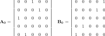(90)

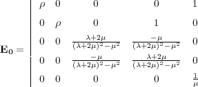(91)

We note that if we let V = E ₀ v, F = A ₀ v, and K = B ₀ v, then Equation  89 takes the form of Equation  92.

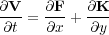(92)

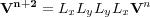
Equations of the form in Equation  92 are called divergence free. Equations of this form are easily split into two much simpler equations which are then solved by splitting methods. The simple conceptual idea is to solve the equation in one direction and then the other, followed by reversing the solution order for the next time stamp. Suppose we let L _x represent one finite difference update using only the x variables and L _y represent one finite difference update using only the y variables. The general process for updating then uses the formula in Equation  93.

(93)

Thus, all we have to do is specify one or the other of the solution schemes L _x, or L _y and completely by symmetry we will have the other. A fourth order in space, second order in time predictor-corrector scheme for L _x takes the form of Equation  94.

Propagation Stability

Each of the various finite difference methods you might construct contains a ratio of the form , where ν is one of the spatial increments Δx, Δy or Δz. It might come as somewhat of a surprise that if this ratio is too large, the propagation scheme it helps define will not be stable. An unstable scheme will eventually produce excessively large numbers and exceed the numerical accuracy of the machine it is running on.

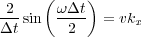
Derivation of a formula that can provide an accurate bound for these ratios requires that we first relate frequency to wavenumber. To do this in a simple manner, we begin with the 1D version of the Lax-Wendroff discrete pressure equation (Equation  17), as shown in Equation  95, where v is velocity.

(95)

To make our life just a bit easier, we assume a solution of the form exp and ignore the higher terms to obtain the dispersion relation in Equation  96 and Equation  97.

(96)

(97)

Although the true dispersion relation for the 1D equation has c = , Equation  97 says that the discrete velocity is greater than the true velocity.

(98)

Thus, to avoid explosive growth, we must have the relation in Equation  99.

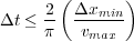(99)

A similar analysis shows that to achieve stable isotropic elastic ( P SV ) waves, we must have the relation Equation  100.

(100)

The important aspect of this analysis is that we cannot choose our time step size arbitrarily. We must use the appropriate version of Equation  99 or Equation  100 to assure that the calculations we perform and consequently the waveform we produce will not grow exponentially.