Algorithmic Differences

Figure  32 shows the basic differences between different classes of migration algorithms. The top left part of the figure is a schematic of a typical curved-ray time migration. Note that this approach uses a single arrival and also uses a single v ( z ) velocity for each output image point. This means is that the curved ray time migration is really a v ( z ) depth migration that uses a completely different model for each and every output point.

Figure 32: Prestack migration differences

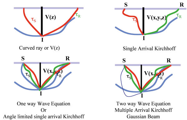
The top right part of Figure  32 conceptualizes a single arrival Kirchhoff depth migration. Here, the single arrival is chosen by shooting rays in a fully three-dimensional Earth model. In this case, the migration is a truly three-dimensional process. In complex media, the forced choice of a single arrival increases this method's sensitivity to rapid and strong velocity variation. It is not surprising that single arrival Kirchhoff depth migration has considerable difficulty imaging below salt structures. Nevertheless, the flexibility of this approach means that it will remain the workhorse of migration velocity analysis for Earth model estimation.

The bottom left part of the figure shows a characteristic multiple arrival migration methodology. Among the techniques that achieve this goal are one-way FKX wave-equation algorithms and multi-arrival Kirchhoff methods that do not allow turning rays. Because turning rays have been eliminated, the methods envisioned in this figure cannot image beyond 90 degrees.

The bottom right part of Figure  32 illustrates a full, or at least nearly full, two-way methodology. In this setting, waves described by all incidence and reflections angles are imaged. The methods that have this kind of capability include full multiple-arrival Kirchhoff algorithms, Gaussian beam methods, and, of course, full finite difference reverse time migration.

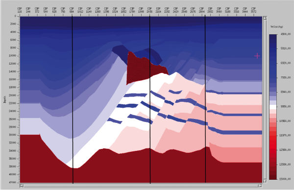
To further understand migration differences, Figure  33 shows impulse responses from two different algorithms at three different trace locations in the velocity model at the top of this figure. The vertical black lines mark the position of synthetic traces from the data set generated over the model. The top row of impulse responses are based on one-way FKX algorithms while the bottom row are based on a single arrival Kirchhoff method.

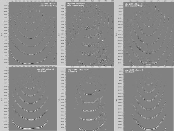
Because the left hand impulse response column represents a trace from that side of the model, the lack of strong lateral velocity variation results in almost identical wave-equation and Kirchhoff responses.

In contrast, the middle column represents a trace with a midpoint directly over the salt structure in the center of the model. Note that while the Kirchhoff amplitudes are comparable to those of the response in the top row, the tremendous number of multiple arrivals and phase changes are quite evident. It is possible to program the Kirchhoff response to almost exactly match the wave-equation response, but the effect is difficult to achieve.

Since the trace used to compute the right hand column is also out of the strong lateral velocity zone, its affect on arrivals is not as noticeable as the center column. Nevertheless, the need to compute a large number of multiple arrivals is still quite clear.

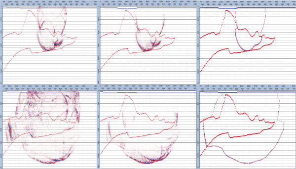
Figure  34 shows the extremely complicated impulse of both the two-way and one-way methods, and demonstrates the need to use highly accurate algorithms in complex geological media. Many people would argue that the smooth structure of the Kirchhoff impulse response on the right is the correct approach. However, the best results are produced using the full two-way method on the left. In some cases, the most pleasing image to the eye is not the best approach to producing a full image.

Figure 34: A simple comparison of Kirchhoff, one-way and two-way impulse responses over the SEG/EAGE AA' data set.