Migration in Depth
This section describes a number of the methods used to perform migrations in depth. In depth migration, reflections in seismic data are moved to their correct locations in space. These methods include both explicit and implicit one- and two-way methods, two-way reverse time methods, Kirchhoff style methods, and plane wave techniques.
Explicit Two-Way XT-Reverse-Time Migration
Perhaps the easiest way to understand migration is to consider what we learned in Equation 2. To produce true zero-offset data, we started with a given model, halved the velocity, computed reflection amplitudes for each point on a reflector, and then simulated explosions at each such point reflector. These simulated explosions were ignited at t = 0. The surface wavefield at z = 0 for all possible recording times, t, became a zero-offset subsection. The trick of halving the velocity was all that was necessary to ensure proper arrival times in our zero-offset experiment. It does not take a lot of thought to see that if we simply reverse this process, we will arrive at an algorithm that will produce an image of the subsurface at the original t = 0.
This "reverse time migration" uses the reversed time data as a source term for a seismic modeling exercise. Thus, the "source" in this case is a multiplicity of traces. In 3D, it would be a common-offset volume where the distance between the source and receiver is zero. Figure 2 is a schematic example of the process. The first and second lines of Figure 2 show what remains as each time slice is propagated into the output image, while the second and fourth lines show the current image at each propagation step. Thus, the upper first and second images in the upper left show the initial condition of the zero-offset wavefield and the subsurface. In actual practice, the initial subsurface subsection would be filed with zeros. Here, we just reversed the modeling images from the subsection on modeling. Note that as the process continues, the final subsurface at the bottom right contains the fully migrated image. All amplitudes in the original recorded zero-offset subsection have been exhausted and are now zero; that is, the entire recorded wavefield has been back propagated into the Earth. Note that in these images, all subsurface reflectors are clearly being imaged from above and from below.

Figure 3 visualizes what happens locally during the process described by Figure 2 and its associated comments. Input traces are reversed in time and fed directly into the modeling algorithm to produce the final image. This kind of method is called an explicit method because it back propagates time-reversed data one step at a time.

Implicit Two-Way XT Reverse-Time Migration
The only difference between explicit and implicit zero offset migration is that the former explicitly employs the mesh shown in Figure 3, while the latter inverts a rather large matrix to obtain the migrated image. The "sources" in both are the time-reversed stacked or zero-offset traces, so the only differences between the explicit and implicit versions involve the implementation.
Two-Way FX Reverse-Time Migration
We need only review our discussion on frequency-domain reverse-time modeling to understand that this frequency domain method must also invert a matrix to achieve its result. Because the 3D version of the matrix M ( ω ) in ???? is so large, this technique has been used infrequently. Research has shown it to have significant advantages in solving inverse problems, but it will probably remain in research environments until sufficient computer power is available to make it practical.
Explicit One-Way XT Reverse-Time Migration
Again, going back to our modeling discussion, it is quite easy to make a one-way migration method. Figure 4 illustrates this point quite accurately. Note that three-dimensional, one-way-reverse-time migration differs from its two-way counterpart only in that the propagating stencil is free of coefficients below the current time or depth slice. Thus, unlike the two-way algorithm, one-way imaging proceeds one time or depth slice at a time. It is precisely this feature that makes one-way wave equation imaging vastly more efficient than its full two-way cousin.

Implicit One-Way XT Reverse-Time Migration
Here we only need to invert the appropriate upper-diagonal matrix to find the imaged solution. Because the process is based on a back-substitution method, it is extremely efficient and therefore much faster than the full two-way-implicit scheme.
One-Way FK Reverse-Time Migration
One-Way-FK-Reverse-Time Migration methods can be divided into FK, phase shift methods, and phase shift plus interpolation methods.
FK or Stolt Migration
In the mid 1970's, R. H. Stolt at Conoco's Ponca City, Oklahoma research facility invented what has become known as Stolt or FK migration, as shown in Figure 5.

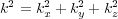
What Stolt recognized was that in a normal zero-offset seismic experiment, we are given time data u ( x;y; 0 ;t ) measured at z = 0, and what we want is the exploding reflector depth data u ( x;y;z; 0). He also understood that if he could compute the depth wavenumber, k z, from frequency, ω = 2 πf, and the x and y wavenumbers, he could produce a very fast FK domain method.
Figure
5 shows how he did migration. The vertical wavenumber
k
z in depth is directly computable from the 2D
dispersion relation
k
2
=
k
x
2
+
k
z
2 where
k
=
 . Because the dispersion relation in Equation
5 holds in 3D,
extension to three dimensions is straightforward.
. Because the dispersion relation in Equation
5 holds in 3D,
extension to three dimensions is straightforward.
 | (5) |
The assumption of constant velocity is the Achilles' heel of Stolt's method. It cannot be derived mathematically unless the velocity is constant, and no method has ever been found to overcome this weakness. However, since it was Fourier-based, it was much faster than any of the other methods of the day. Researchers quickly tried to get around the constant velocity issue.
Phase Shift Migration
The phase shift method shown in Figure 6 was based purely on reverse-time modeling. It was one of the first approaches to successfully remove the constant velocity criteria imposed by the Stolt approach. It was also the first and, perhaps until very recently, the only method that was capable of imaging up to 90 degrees. The phase shift approach was invented by Jeno Gazdag shortly after the Stolt method appeared. What it does, in effect, is to successively apply the Stolt method to each slice in a Earth model where the propagation velocity varies only vertically. Thus, it is a recursive technique that repetitively applies the formula for k z in Figure 5 to each constant velocity depth slice in the v ( z ) model. It begins at zero depth ( z = 0) and proceeds until the desired depth is reached. As long as the Earth's velocity varies only vertically, it does a remarkably good job of imaging steeply dipping events. This approach can be modified to include at least some two-way propagation, so it is also very versatile.

|
Phase Shift Plus Interpolation Migration
As discussed in the chapter on seismic modeling, phase shift plus interpolation (PSPI) modeling is easily adapted to produce a phase-shift-plus-interpolation style reverse-time migration, as shown in Figure 7. The sources in this case are again the time reversed traces and the result is a depth image of the zero-offset input data.

One-Way FKX-Reverse-Time Migration
One-way FKX-reverse-time migration methods can be divided into split-step and phase screen methods.
Split Step Imaging
The split-step imaging method is a direct application of the split-step modeling method in Equation 2. Explaining this method in considerable detail is beyond the scope of this book. For the purposes here, it is enough to say that the method splits all downward propagation between the FK and FX domains.
Phase Screen Migration
The so called phase-screen method, as envisioned by Ru Shan Wu at the University of California at Santa Cruz, is discussed briefly in Higher Order FKX Methods. This method, when compared to the split-step approach, is based on an improved set of approximations for utilization in the FX domain.
Kirchhoff Style Methods
Kirchhoff migrations are a method of seismic migration that uses the integral form (Kirchhoff equation) of the wave equation. Kirchhoff style methods can be separated into single-arrival methods and multiple-arrival methods.
Single-Arrival Kirchhoff Migration
In single arrival Kirchhoff depth migration, as shown in Figure 8, either a direct finite difference solution to the Eikonal equation or full 3D raytracing is used to calculate exact traveltimes from the source/receiver point to the output image point.

Because Eikonal-based methods are generally able to calculate only first arrivals, they are no longer popular as part of the general depth migration methodology.
However, raytrace methods facilitate the calculation of multiple arrivals, and the selection of those arrivals better serves the migration process. Typical arrivals of this type are maximum energy, minimum distance, or minimum velocity. In areas with strong lateral velocity variations, such as salt regimes, the minimum velocity methodology is considered to be optimum since they avoid headwaves caused by proximity to salt or other high velocity structures.
The utilization of a single arrival in Kirchhoff depth migration technology is one of the chief reasons these methods cannot image below complex structure.
Multiple-Arrival Kirchhoff Migration
When we use all of the possible arrivals, as shown in Figure 9, we can achieve a superior result to what is achieved with the single arrival approach. While multiple arrivals complicate the migration algorithm and generally make it more computationally costly, the benefit of including more arrivals usually outweighs the increased cost.

Plane-Wave Migration
Plane-wave migration methods can be divided into pure plane wave methods, beam stack methods, and Gaussian beam methods.
Pure Plane Wave Migration
The hand migration discussed in the chapter on historical methods and displayed in Figure 5 is in actuality one of the first plane wave migration techniques. The constant velocity trigonometric solution in that figure provides the formulas for calculating the migration time, τ, and the lateral shift, x, to determine the migrated position, S 0.
Figure
10 shows how you can avoid the constant velocity assumption completely. In this figure, the
 measured from the unmigrated data, together with the near surface velocity, determines the cosine of
the plane wave takeoff angle,
θ, at the zero-offset location of the reflected arrival from
the steeply dipping structure. If we shoot a ray with this takeoff angle into the subsurface model
and continue it until the recorded time at
A is exhausted, the orthogonal to the ray will be the dip of
the reflected event and the position of the end of the ray will be its location. Repeating this process
for every estimated dip ultimately produces a full migration of the recorded zero-offset or stacked
subsection.
measured from the unmigrated data, together with the near surface velocity, determines the cosine of
the plane wave takeoff angle,
θ, at the zero-offset location of the reflected arrival from
the steeply dipping structure. If we shoot a ray with this takeoff angle into the subsurface model
and continue it until the recorded time at
A is exhausted, the orthogonal to the ray will be the dip of
the reflected event and the position of the end of the ray will be its location. Repeating this process
for every estimated dip ultimately produces a full migration of the recorded zero-offset or stacked
subsection.

Beam Stack Migration
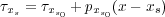
Kirchhoff methods are converted to a beam or slant stack approach by simplifying the manner in which traveltimes are calculated. The idea is to try to use the distance from a central source or receiver to calculate another traveltime at a nearby location. In two dimensions, the formula is something like that shown in Equation 6, where τ x s 0 is the raytraced traveltime from the central location, x s 0, and p x s 0 are suitably chosen scalars.
 | (6) |
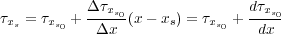
Noting that p x s 0 must have units of time over distance, we can easily infer that this value must tell us how τ x s 0 changes incrementally versus an incremental change in the central source position. That is, p x s 0 must have the form in Equation 7, which is just the derivative (gradient in 3D) of the traveltime with respect to source position.
 | (7) |
Traveltimes at a position close to the central point can then be calculated from Equation 8.
 | (8) |
Equation 9 performs a standard zero-offset Kirchhoff migration in 2D, where A is a traveltime correction factor, τ x s ( x;z ) is the traveltime from the surface location x s to ( x;z ), and D ( x s ;t ) is the zero-offset data to be imaged as I ( x;z ).
 | (9) |
The basic ideas for this kind of traveltime computation is shown in Figure 11.

Inserting the formula for calculating τ x s results in Equation 10.
 | (10) |
Equation 10 suggests that we can perform this operation in two independent steps. First, we calculate the slant stack of our input zero-offset data, D ( x;t ), using Equation 11. Then we simply Kirchhoff migrate this slant stack bundle using Equation 12, where the sum is taken over all x s that are sufficiently close to x s 0. The image I ( x;z ) is then just the sum of all the bundles.
 | (11) |
 | (12) |
Since the slant stack can be calculated independently of the migration, and since the derivative of the traveltime can be calculated during the raytracing, the computational cost of performing the necessary steps prior to the migration stage is only slightly greater than that required for a standard Kirchhoff migration.
On the other hand, since the entire slant stack bundle replaces many traces in the migration process, Kirchhoff-beam-stack methods can be significantly more efficient than their traditional straight-forward implementations. Typically, these Kirchhoff-beam-stack migrations are about 10 times as fast as a traditional Kirchhoff approach.
Gaussian Beam Migration
Figure 12 demonstrates graphically how we can construct a significant portion of the required impulse response for a zero-offset trace using what are called Gaussian beams. The mathematics associated with Gaussian beams is beyond the scope of this book, but the concepts are worth some explanation. Although somewhat of an over-simplification, we can think of a Gaussian beam as being equivalent to a phase shift calculation using a v ( ρ ) velocity function extracted using the arc-length along the ray, ρ, as the depth parameter.

Several corrections to this phase shift are made to ensure that the process works correctly. First, as the ray calculations proceed, two special functions are calculated at each increment, Δρ, of the arc length. These functions provide the necessary amplitude decays parallel and orthogonal to the ray at any given location. Second, the beam is weighted with the normal Gaussian function to ensure that the sum of all such beams accurately represents the true impulse response of the migration operator. The result of applying the corrections is called a Gaussian beam, and its amplitudes are then summed into corresponding subsurface locations on either side of the central ray. The sum of all such beams produces the completed impulse response.
