Horizon-Based Velocity Analysis

So the question is: Do we ever need horizons?

In some sense, the answer is driven by how well we can flatten the gathers we output from the Deregowski loop. It is great when the painless method does a good job of flattening the gathers because horizons certainly create a plethora of problems in an iterative scheme for velocity estimation. We would like to avoid these problems in all situations. Horizons change shape and position every time a new Earth model is part of a re-migration of the original input data. The processor is then either forced to reinterpret a new set of horizons or to edit the existing set prior to another iteration of velocity analysis. It would certainly be nice never to have to worry about horizons. There are also geologic environments where horizons are just as useless as the painless approach in those environments, but it is also probably true that in this kind of regime, nothing will produce acceptable results.

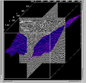
There are certainly many geologic settings where the use of horizons is absolutely necessary. Horizons are essential when strong, visible velocity anomalies, such as salt domes and sills, are present. The tops, sides, and bottoms of these visible bodies are interpreted, defined as horizons and inserted into an existing Earth model. Figure  21 shows how the top of salt is interpreted in a salt flood exercise.

Horizons are probably also essential when velocity anomalies are invisible. In this case, we cannot interpret the tops, sides and bottoms, so horizons above and below the suspected area are the only option. In certain geologic settings, most notably in areas with strong carbonate bedding, fast velocities within relatively thin sections require utilization of interpreted horizons to produce adequate estimates of the velocity within the bedding planes. When data-based estimates are insufficient, horizons may also be useful as control surfaces allowing constant velocity insertion between specific layers to define a more accurate Earth model. Perhaps the most important setting where horizons are required is when it becomes clear that the painless approach has failed miserably. In this case, it is probable that an attempt to apply tomographic inversion will also be recommended. However, there are always exceptions to almost every rule. In geologic environments where subtle velocity variations are not easily seen, we may have to resort to more extreme approaches. This would definitely include very fine horizon based velocity model construction along with full utilization of tomography.

Figure  21 is an illustration of the interpretation of horizons on top of a base of salt. This kind of interpretation is also necessary for certain kinds of residual tomography. Typically, a reasonable set of horizons provides tomographic inversion with precisely the information necessary for success. It is not necessary to be as accurate as we might be for prospect generation, but it is necessary to define as many horizons as possible.

Once horizons have been defined, velocity picking can be done along the horizons themselves. While this should produce horizon consistent velocities, vertical updating through the Dix equation is still necessary to provide the required interval velocity estimates above the horizon under analysis.

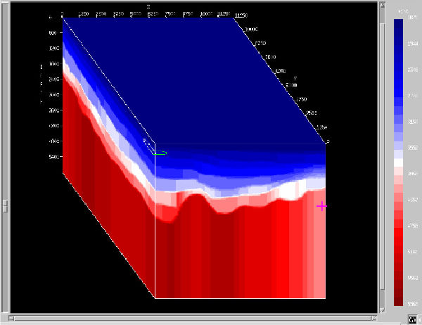
Figure  22 shows the kind of model produced from a typical horizon based approach. It is difficult to believe that the blocky nature of this model is realistic. Because they are high frequency approximations, raytracers have considerable difficulty calculating accurate traveltimes unless the model is smoothed. The only real way to avoid the blocky nature evident in this image is to interpret a large number of densely spaced horizons or to insert a large number of invisible horizons between relatively sparse sets. Interpreting a large number of horizons requires a considerable amount of human time and cost. Interpolation of a fine set of horizons between a sparse set seems to be moving back toward a more painless methodology. However, in geologic situations where compaction plays an important role in vertical velocity variation, forcing the velocity structure to follow horizons when they are not the chief defining factor can be disastrous.

Figure 22: A horizon based velocity model

In Figure  23, we see a set of gathers that have been through several iterations of vertical or Dix updating. Note that the gathers on the right are reasonably flat while those on the left are not flat. Because these gathers produce poor images when stacked, this phenomenon cannot be improved by traditional horizon-based vertical methods. This three-dimensional effect was ultimately resolved only through careful application of tomography. While there are many approaches to tomography, recent experience has shown that residual methods work the best. Residual approaches are usually applied only after an initial migration velocity volume is available. They also normally require reasonable information about local dip, which can be obtained from a horizon-based approach, or by direct estimation of the local dip from the current image, or from specific geologic knowledge. Since horizon-based methods tend to offer better accuracy than direct automatic estimation, we restrict our attention to that methodology. Note that this implicitly assumes some form of geologic interpretation of the region or area under study.

Figure 23: Non flat gathers.

Figure  24 shows a typical horizon-based velocity analysi–velocity model building workflow. This sequence of processes is almost identical to that in Figure  16, except that velocities are "snapped" to user-defined horizons rather than to an equally spaced set of flat horizons. Perhaps one benefit to this kind of analysis is that once the process has reached a stationary point, all the necessary information required to apply tomography is in place.

Figure 24: A horizon based velocity analysis workflow