Swing Arms

This section presents additional information about swing arms, which were mechanical devices enabling you to migrate dip data.

Isopachs and Isochrons

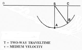
In view of the comments in the preceding sections, one conclusion becomes quite clear—any apparent reflection on any given trace could have come from any point on an equal traveltime subsurface isopach. An equal traveltime isopach is that set of points in the subsurface whose traveltimes from the surface and back (two-way times) are identical. Figure  27(a) shows an equal traveltime curve in a constant velocity medium for zero-offset reflections. Clearly, if all we have is a zero-offset trace, we can only infer that the reflection could have come from any point on the equal-traveltime isopach defined by the reflection time.

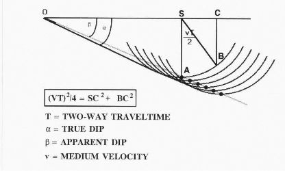
Figure  27(b) provides the simplest mathematics defining an equal traveltime curve. It also shows how the apparent horizon (dotted line) is imaged as the envelope (dark solid line) of a set of equal traveltime curves.

For any given arrival on a recorded seismic trace, all potential locations from which this arrival could have been reflected lie on a circle with the source point as the center and the velocity-time depth as the radius. If we trace out a circular isopach for each source, the envelope of all such isopachs will be the location of the actual reflecting surface. Since the velocity is assumed to be constant, these circular isopachs can also be thought of as isochrons, or curves and surfaces in time rather than depth. Regardless of terminology, a swing-arm built on this principle has a significant advantage over hand plotting each vector to migrate the given dip data. An entire zero-offset stick map could be migrated with a constant velocity without every resorting to any calculations at all. Of course, the constant velocity assumption meant that the results might not be accurate, but they could be redone quickly. A different constant velocity could be used for each surface position to at least make the resulting migrated stick map as close as possible to subsurface truth.

Operators

Figure  28 provides the time response on the surface for a single point reflector in the subsurface.

Figure 28: Operators and operator migration—Point reflector zero-offset response

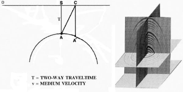
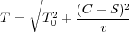
Every time on this time domain curve is the two-way time from the surface source to the point reflector and back to a receiver at exactly the same location as the source. The time recorded at A 0 below C is actually the time it would take for sound to travel from a source at C to the point reflector below S and back to a receiver at C. As indicated in Figure  28 for a constant velocity medium, the set of all such times can be calculated quite easily using Pythagorus' theorem.

(6)

In a more complex velocity medium, the curve would not be a circle, but would still represent the zero-offset reflection times from the point reflector. Zero offset responses are quite easy to calculate, and raytrace modeling is fully capable of calculating such responses in virtually any medium.

The operator approach to migration computes an operator curve, intersects it with each input trace, selects the amplitude at the intersection time, and then adds it to the image point or output location on or near the top of a downward facing frown. In actuality, this is completely equivalent to the previous diffraction-based approach. They both produce the same result, but this one is a bit more difficult to understand. Figure  29 shows an amplitude at A being moved to the top of the zero-offset response curve and added to the reflection point location at B. In general, all the amplitudes that intersect the operator would be summed into the top of this curve at point B. However, the only non-zero amplitude point that we can see is at A. As the process continues, each and every point on the apparent or unmigrated reflector is moved to the top of the associated zero-offset response curve and added to the appropriate spot on the migrated image represented by the solid line in Figure  29.

Figure 29: Operators and operator migration—Zero-offset response or operator migration

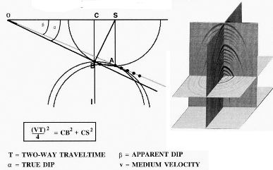
The three-dimensional figure on the right illustrates all the amplitudes from surrounding traces that contribute to the trace in the middle. These frowns are called operators, but they are really the modeled response of a point reflector at some subsurface location. The important thing is the process and not the shape of the zero-offset response.

This approach to migration is somewhat more difficult to understand than the spray approach of the previous section. Why it works should become much clearer in the chapter on seismic modeling. However, one thing should be clear, it is based on modeling a point reflector and not on the possible locations from where the reflector might have come.