Shot Profile Hand Migration in Two Dimensions

Picking traveltimes from a short-offset trace to approximate zero-offset arrivals and thereby produce a zero-offset section works well when neither the velocity nor the geometry of the local formations vary dramatically. It breaks down when velocity variation is strong, when the structure of the subsurface horizons is complex and when assuring that the current pick is on the same formation as the last pick is difficult.

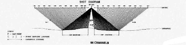
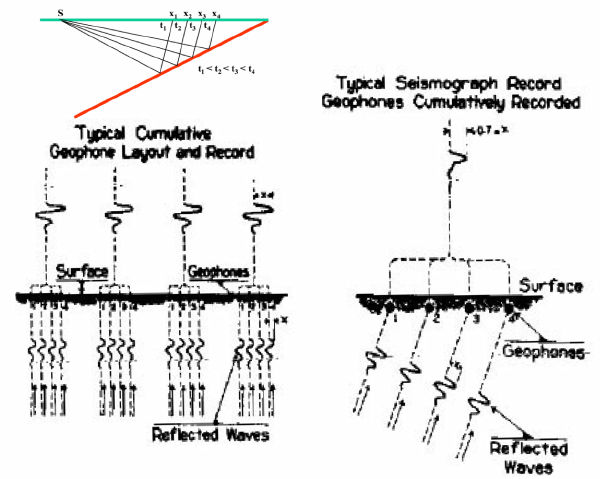
The first approach to alleviating at least some of these problems was to increase the number of geophones in each shot profile. Instead of using a handful of receivers on one side of a shot, "split-spread" shooting, as shown in Figure  9, became prominent. After each shot was recorded into multiple receivers, one half of the receivers were picked up and moved to produce a new split-spread array for the next shot. For example, in the diagram in this figure, the receivers on the left would be moved so that the left-most receiver is just to the right of the right-most receiver. A new source would be discharged and recorded into the newly positioned array. As this process continued, complete coverage of the subsurface reflector is accomplished. As shown in the left hand trace graphic in Figure  10, trace-to-trace correlation is now much easier, and subsurface mapping is supposedly simplified.

Figure 9: A typical two-dimensional shot diagram from the mid 1960's to around 1975. These were used in split-spread shooting arrangements.

Figure 10: Detecting dip. The amplitude and direction were defined by a slant stack.

A key question that needed an answer was what does dip really look like on a shot record with a large number of receivers. Could shot-record dip be used to estimate the location of the reflecting horizon?

These questions were not focused so much on dip, but on whether or not you could estimate the dip from the shot profile and then figure out where the reflection came from. Figure  10 shows Rieber's 1936 solution to the question of estimating dip. He delayed each shot linearly (right hand side of the figure) and summed up the amplitudes. When a large amplitude was found, the delay required to find it defined the emergence angle, and so gave insight into both the arrival direction and the amount of subsurface dip that produced it. He was probably the first to recognize the importance of summing over lines (slant stacks) to reduce the problem to one of simply detecting an amplitude.

Unfortunately, I am not aware of anyone who took advantage of Rieber's methods in any detail during his day. It was not until the advent of modern computers that his method came to the forefront in the form of plane-wave or beam stack approaches to imaging. However, using information from a shot profile still became a viable approach to more accurate subsurface mapping.

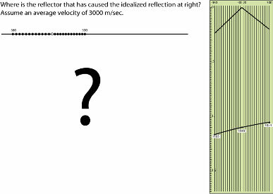
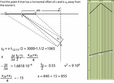
Figure  11 shows what an aspiring geophysicist named Klaus Helbig was given as a test in 1952. It was his introduction to geophysics. He is a well known German geophysicist who is still alive at this writing and is a wonderful source of historical information about how geophysics was done prior to the advent of powerful computers. I am indebted to him for many of the figures and exercises in this section. Figure  11 shows a synthetic shot profile on the right. The problem, given an assumed velocity of 3000 meters per second, is to find the reflection point that generated the shot record on the right. As described in Figure  12, the problem is easily solved by applying Pythagorus' theorem, and Figure  13 provides the numerical answer to the problem. This calculation requires close attention to the different signs, but essentially everything still moves up dip. Even at the modest production rates of the fifties, it was unavoidable that errors crept into the several hundred calculations that had to be performed by hand. As Helbig says:

Figure 11: A test for an aspiring geophysicist.

Figure 12: Klaus Helbig's solution to the problem of Figure  11.

Figure 13: The numerical solution to the problem in Figure  11.

It is worth noting that we can use virtually any two picks from the shot record displayed in Figures 11, 12, and 13 to perform a migration. Such picks can be from any pair of traces within the shot profile, so, technically speaking, we can migrate the shot record in a very detailed manner. It is also worth mentioning that what is happening is shot-by-shot migration. It was done by humans as opposed to a digital computer, but it is still a shot-by-shot or shot profile migration.

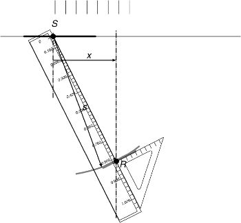
Performing the computations involved in migration by hand is clearly difficult. Even in two-dimensions, this process was fraught with error. As a result, there was a strong push to automate the process to be able to choose well locations quickly and more accurately. One of the first such devices, as shown schematically in Figure  14, might best be described as a plotting device.

Figure 14: A simple machine for drawing reflectors at positions determined by the solution to Klaus Helbig's "thought problem."

As drawn, it cannot directly calculate the value of x (Equation  1) in Figure  12, but given a bit of experience by the interpreter, it can produce very accurate stickmap interpretations of true subsurface horizon locations.

(1)

Again, according to Klaus:

While it is not really a migration machine, it does foretell the kind of device that would follow to reduce the computational complexities associated with the constant velocity and straight ray formula of Figure  12.