Aliasing
Aliasing happens when the frequency of repetition is too fast for the true nature of the repetition to be recognized. For example, everyone who has ever watched an old American Western movie has seen wagon wheels, maybe like those in Figure 5, spin diametrically opposed to the direction of travel (backwards). This occurs because the thirty-frame per second sampling rate of the movie camera is incapable of resolving the faster rate of the wheel spin. The net result is that the wheel appears to spin at a slower rate in the wrong (backwards) direction.

For our purposes, spatial aliasing in seismic exploration makes it impossible to correctly distinguish and image dipping events at their true position and angle. Many people argue that the mathematics of sampling is incorrect because they believe that if the human eye can recognize the correct pattern, the more mathematical migration algorithms should also be able to do so. But our brains make the event appear continuous, and handles it from there, while discrete mathematics cannot do this. The mathematics of discrete migration algorithms make strong demands on what kind of data they can handle because they cannot make the data continuous before they process it. Consequently, both acquisition design and the imaging algorithm must take aliasing into account. In some cases, the algorithm can be designed to handle any aliasing problem or issue automatically and directly. However, when this is not the case, aliasing must be avoided during the acquisition process itself. The elimination of aliasing ensures that dipping events are imaged as optimally as possible.
Data acquisition parameters play an important role in subsequent imaging exercises, while imaging algorithms vary considerably in their sensitivity to acquisition parameters. Understanding the impact of acquisition parameters on imaging techniques is the key to producing superior images.
Many geophysicists believe that there is some magic level of sampling, or that the sampling rules seemingly demanded by acquisition and processing are unnecessarily strict. The basic idea that the human eye is better than the computer at being able to see through under-sampled data is probably true. However, ensuring that any given imaging application produces the most optimum results limits both the kind and style of the acquisition method. For the most part, data must be sampled sufficiently finely to ensure that the imaging algorithm can image target objects without loss of dip or image quality.
Figure 6 provides simple, conservative formulas relating the important parameters that affect the relationship of dipping reflectors at their true subsurface position to their apparent dip on a two-dimensional seismic recording when the source and receivers are coincident and the velocity is constant. The relationship between apparent dip, as specified by a change in time versus a change in space, coupled with Shannon's sampling theorem, tells us when to expect and how to handle potential aliasing caused by spatial sampling intervals.
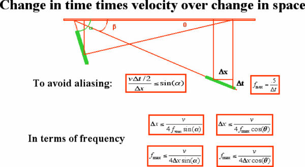
The trigonometric sine function of the true dip of the subsurface event turns out to be the ratio of half of the relative change in two-way time of the event at its apparent position, Δt, to the spatial range over which the time change takes place, Δx, multiplied by the assumed constant velocity of sound in the medium.
After this simple concept is understood, it is straightforward to use the Nyquist relationship between time sampling and frequency to rewrite the basic formula in terms of frequency. The Nyquist relationship states that a signal must be sampled at a rate greater than twice the highest frequency component of the signal to accurately reconstruct the waveform; otherwise, the high-frequency content will alias at a frequency inside the spectrum of interest.
Note that fixing any three parameters in the variety of formulas rewriting the basic formula produces provides a bound for the fourth. In 3D, it is important to do the calculations based on the largest spatial interval in the data set, Thus, if we want to make sure that we can image a given set of dips at a given frequency and velocity, we must make sure that the data has been recorded at the correct spatial spacing, or we must migrate it at the proper sampling interval.
You should understand that these are conservative formulas. The fact that velocities vary helps the imaging process because, in this kind of medium, ray bending improves the ability to image steeper dips. In precise mathematical terms, note that:
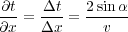 | (1) |
We all claim to understand the idea that when we sample a signal at a fixed even increment, the resulting set of samples can be used to reconstruct the original signal completely, but only up to a fixed frequency determined by the sampling rate (that is, the Nyquist frequency). Thus, if we sample at 250 samples per second (in other words, 4 milliseconds per sample), the highest possible frequency we can record correctly is 125 Hz, or exactly half the sampling rate. Note that in this case, the Nyquist frequency is determined equally from 250 or half of 1.0/.004. Thus, 125 = 1.0/.008. A similar equivalence is available for surface sampling parameters. If lines are spaced at 100 meters, the spatial Nyquist frequency in the line direction is 1.0/200. This Nyquist frequency specifies the maximum wavenumber or wavelength that can be safely recovered from the surface sampled data in the line direction.
Figure 7 shows a schematic of a single plane monochromatic wave front traveling at a slight angle relative to the vertical. The wave front on the right is recorded in time, while that on the left is recorded in depth. The wave front in this case is propagating in a constant velocity medium and is characterized by its vertical and horizontal wavenumbers, or their reciprocal wavelengths. The vertical wavenumber, k 0, is completely determined by the frequency, w, and the velocity, v. In contrast, the horizontal wavenumber, k x, is impacted by the angle of propagation. Later, we will see that this dependence on angle can be used to specify a simple migration algorithm.
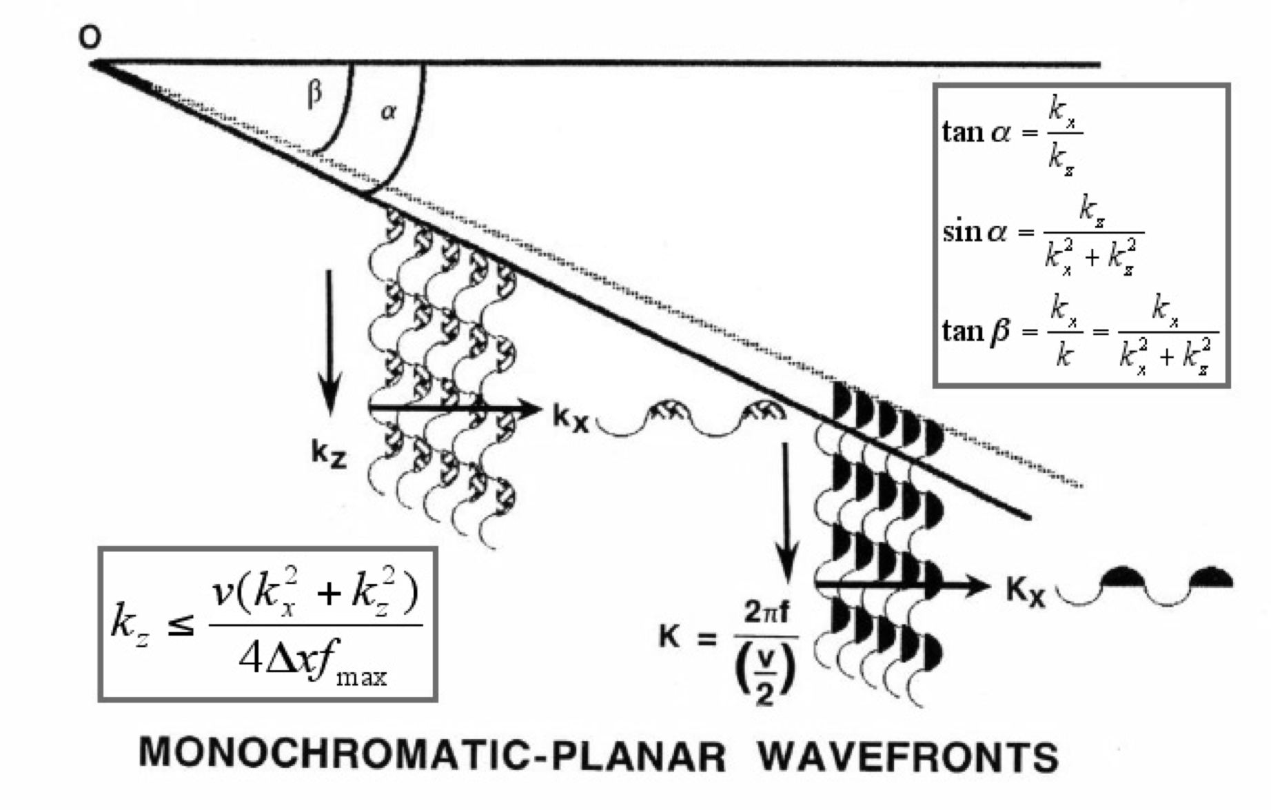
Figure 7 also shows the relationship between monochromatic wavefronts true dip. The figure shows how the trigonometric functions relating apparent dip to true dip are expressed in the frequency domain. The most important formulas say that the sine of the true dip angle, α, is equal to the tangent of the apparent dip angle, β.
It is important to note that in the real world, this means that we must consider our measured seismic data to be digital in character, since the sources and receivers are at discrete locations. Since modern data is also digital in time, reflection seismic processing today is purely digital. Since wavenumbers of propagating plane waves carry information about the angle of propagation, this suggests that there will be some issues with regard to the aliasing of dipping subsurface reflectors. The impact of aliasing on our ability to image subsurface events will be discussed in subsequent sections.
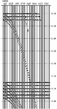
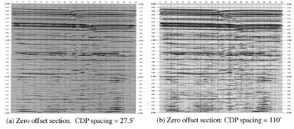
Aliasing appears in many ways. Figure 8 demonstrates the appearance of aliasing on zero offset sections. Here we see the difference between sampling at 27.5 feet and 110 feet. The figure on the left at 27.5 feet is clearly less aliased than the one on the right at 110 feet; that is, the section on the left has been sampled sufficiently finely to almost completely eliminate all aliasing for this level of dip. The section on the right was constructed by simply eliminating traces from the one on the left. Evidence of aliasing is represented by the grainy appearance and by the areas where events that follow some hyperbolic-like trajectory appear more like a single flat event.
The synthetic CDP in Figure 9 is a normal moveout corrected CDP or midpoint gather with both flat and hyperbolic arrivals. It demonstrates a form of aliasing that occurs when the moveout of an event is so strong that the recorded spatial sampling cannot handle its rapidity adequately. This means that events can be aliased in offset even when all dips are perfectly sampled in space. This figure shows a synthetic (raytraced) CDP with multiples that are aliased in offset. While the human eye has no difficulty recognizing the pattern of these events, many noise suppression and migration algorithms will treat these events in a predictable, but incorrect manner. For example, a Radon transform is not be able to completely remove the event from the record.