1954-1959: Dips, Swings, and Special Machines

The year 1954 might have seen the biggest technical leap of all, but certainly the period from the mid to late 50's would have an tremendous impact on seismic imaging.. J. G. Hagedoorn's 1954 () explanation of "A process for seismic interpretation" appears and, as I said in the introduction, becomes one of the foundational papers on seismic imaging. In this paper, Hagedoorn introduces a "string" or "ruler and compass" method for finding reflections as an envelope of equal traveltime curves. This method clearly invokes the by then three-hundred year old principle of one of Hagedoorn's illustrious countrymen, Christiaan Huygens. According to legend, Huygens formed this principle after observing what happened when a line of balls was dropped into the Zuider Zee. Whether true or not, the image of the balls in the water conveys exactly the correct picture of what happens in migration This principle as embodied in Hagedoorn's work was to give birth to the Kirchhoff or "diffraction stack" method several years later 2001 (); 1999 (). In the modern world, the Kirchhoff method in all its various forms has proven to be one of the most flexible and robust approaches to seismic imaging. In addition to Hagedoorn's work, Harry Mayne, 1962 () was beginning the procees of obtaining a patent on the CMP stack that when fully accepted would dramatically facilitate full scale computerized seismic migration. These two developments are certainly the foundation on which migration algorithms of later years were built. It is also known 2004 () that about this time, Geophysical Service Incorporated (GSI), Texaco, and Mobil had a joint effort to develop a digital recording system. Although digital filtering and signal analysis was the primary focus, the consequent development of digital computers would have an enormous impact on seismic imaging.

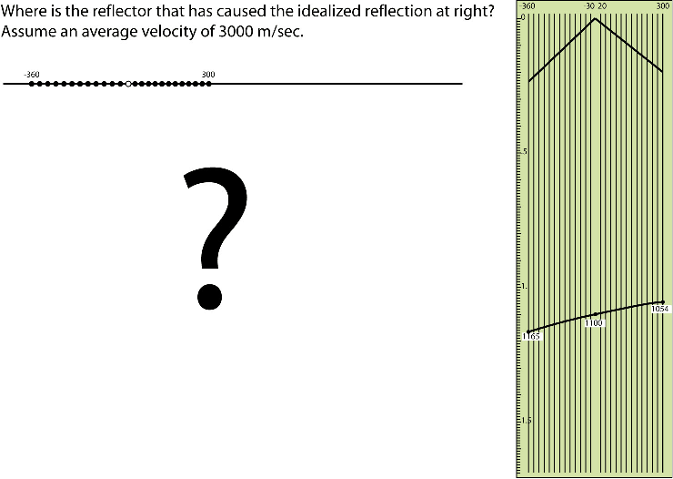
In 1954 computerized Kirchhoff could only have been a dream, but the race was on to design and construct machines capable of moving or "migrating" a given reflection to its proper spatial position. Many successful attempts were made to construct such devices, but because of the imposed secrecy much of what we know about these early "analog migration computers" is hearsay and folklore. Fortunately, Klaus Helbig 2004 () and John Sherwood 2004 () were around then and are still around today. I'll start with Klaus. Klaus had just begun his career at Seismos in Hannover, Germany in 1952 under the guidance of Gerhard Schulz. His first task was to solve the problem in Figure 16. In his own words he describes receiving his first task:

In 1952, I joined an exploration company (Seismos, Hannover) to work on their amplifiers. But first I was given into the hands of a party chief (Gerhard Schulz) for a basic training in the state of the art. To this day I am convinced that he hoped that I would fail. The point never came up since I found the answer quickly.

In Figures 17, 18, and 19 the problem is solved and curved rays provided for. Figures 20 through 25 provide not only a schematic for a reflector plotter but the entire foundation for the develop of a migration machine as realized by Musgrave 1952 () in Figures 26 and 27. Klaus' comments with respect to these figures are included in the figure captions. Apparently the goal was the refinement of an existing migration machine, or what was called a "swing arm" machine here in the states. Again we see another analysis of dipping events and the immediate development of an approach to put the reflection from dipping beds in their proper place. Klaus states:

The machine was operating when I joined the crew in August 1952. Together with the inventor I added some minor improvements. The machine was developed by the party chief entrusted with my geophysics education, and the two of us spent over the next month more time improving the machine than getting me educated. In September I left to join the technical department.

Klaus1 Figure 16. A test for an aspiring geophysicist. Klaus Helbig's 1952 introduction to Geophysics.

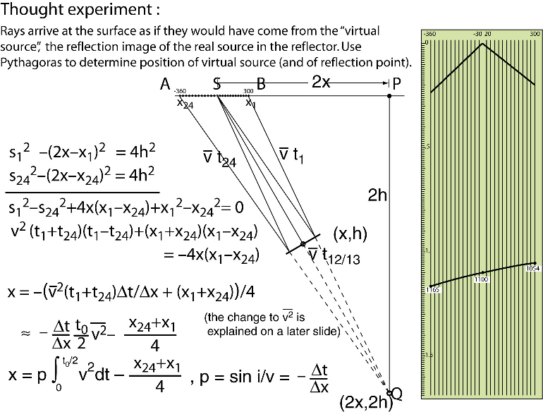
Klaus2 Figure 17. Klaus Helbig's presentation of the solution to the problem of the previous figure.

The explanation for Figure 17 goes like this:

Consider the two right triangles and . and are equivalent to the travel paths from to and to , respectively. The common side is twice the depth of the reflector. The third sides are, respectively, and . Write down the Law of Pythagoras for both triangles and subtract the two equations to eliminate . Arrange to get an expression for . The expression consists of two terms:

• The rightmost term is a quarter of the sum of the horizontal coordinates of the first and the last geophone. It vanishes for a symmetric spread and thus can be regarded as a correction for the asymmetry of the spread. (Today, practically only end-on spreads are used, the asymmetry correction would never vanish).
• The leftmost term consists of the negative horizontal component of the time gradient, and the product of the square of the velocity and a quarter of the sum of the times at the first and last geophone, respectively. The minus sign in front of the time gradient (and in the definition of the ray parameter p) is due to the use of a reflected wavefront: if the downgoing ray is in the positive quadrant , we have on the upgoing rays .
• One quarter of the sum of the times on the first and the last geophone can be replaced with half the time at the center of the spread.
• The final change from the square of the average velocity to the average of the squared velocity accounts for the deviation of the ray from a straight line, as will be explained on a later slide.

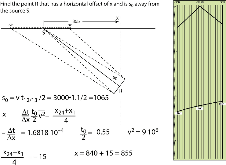
Klaus3 Figure 18. An answer to a tough problem. This calculation requires close attention to the different signs. Even at the modest production rates of the fifties, it was unavoidable that errors crept into the several hundred calculation by hand that had to be carried out. Other companies must have had their way of dealing with this problem. In our company a two-dimensional slide rule was used. While it was not absolutely fool proof it simplified the calculations drastically and forced the operator to be consistent. Consistent sign errors are more easily detected than random errors.

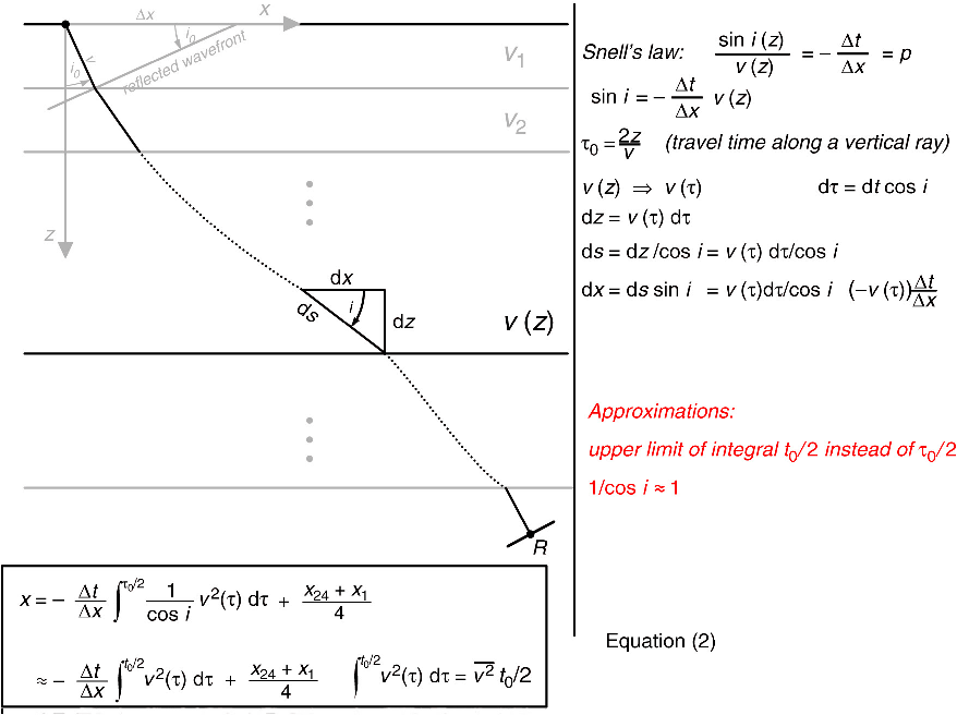
Klaus4 Figure 19. Corrections for curved rays. Up to now the rays were implicitly assumed to be straight. As long as the velocity depends on depth only, it is easy to incorporate curved rays by solving the problem layer-for-layer and then integrating. Since depth is unknown afore hand it is more consistent to integrate over VERTICAL time, I.e. over the time along a vertical ray. While specific cases can be solved exactly, the general case of arbitrary dependence of velocity on depth requires the two approximation shown in red in the figure.

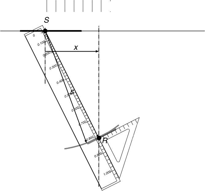
Klaus5 Figure 20. A schematic for a reflector plotter. A temporary vertical line is drawn at horizontal distance down to the (expected) position of the reflector element. A ruler graduated in distance traveled for given times (times are displayed on the scale) is placed so that the zero-mark is at the source and the actual traveltime at the intersection with the temporary vertical line. With the ruler firmly held in place, a small set square is placed against the ruler to draw the forward part of the reflector elements. The set square is graduated at half the scale of the rest of the drawing. This simplifies the drawing of the lengths of the parts of the reflector elements (about half as long as the corresponding surface spreads.

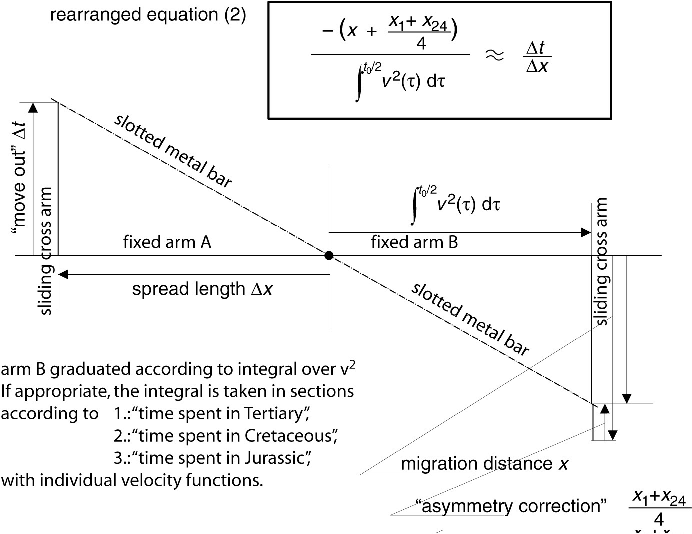
Klaus6 Figure 21. Principle for a machine for event migration. The negative migration offset not corrected for the asymmetry of the spread stands in the same relation to the integral over the squared velocity as the time difference to the position difference. The different parts of this relation are assigned to corresponding sides of two similar triangles.

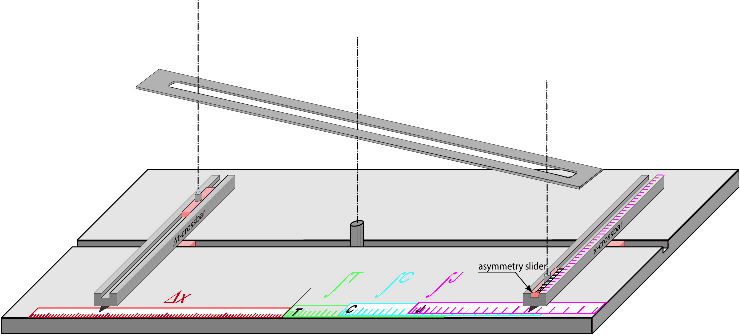
Klaus7 Figure 22. A machine design. The dimensions of the machine were about 1m by 70 cm. Since most reflections were visible on all 24 traces, the delta-x setting and the asymmetry setting remains generally constant at least during the calculation for a seismogram.

Klaus9 Figure 23. The mathematics for a wavefront chart.

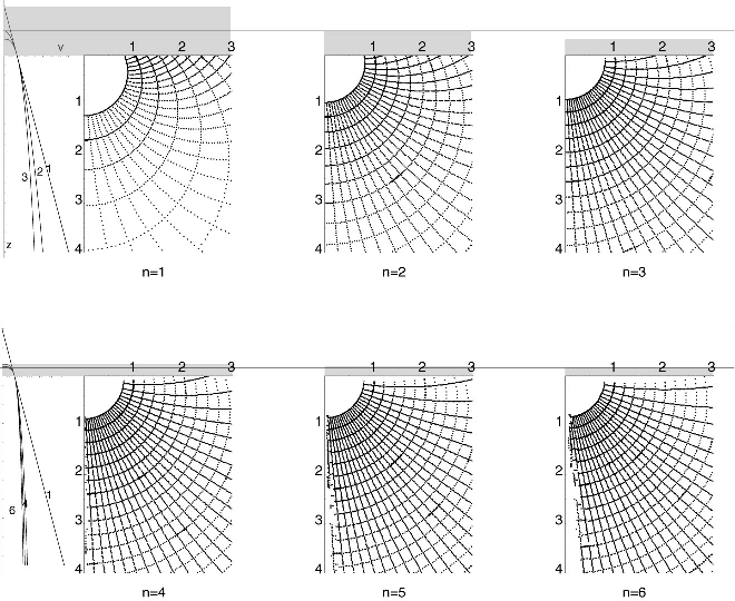
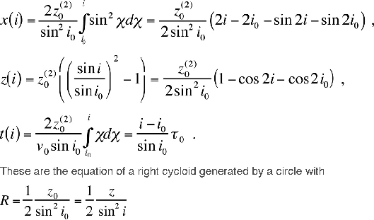
Klaus8 Figure 24. Wave front charts for velocity functions (v/v0)n = (z+z0)/z0. n=0 constant velocity, n=1 standard chart (constant velocity gradient, rays are circles, fronts are spheres). n=2 is more realistic, but in the pre-computer days difficult to generate. Albert Musgrave 1952 () invented a machine to construct rays in such a medium. No machine seems to have survived.

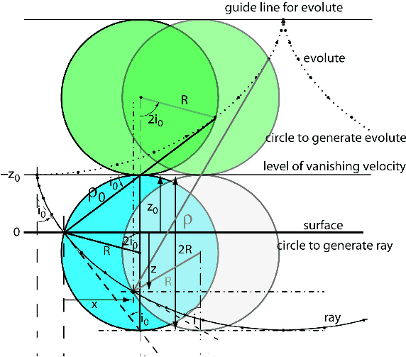
Klaus10 Figure 25. The basis for A. W. Musgrave's migration machine used by Mobil Oil.

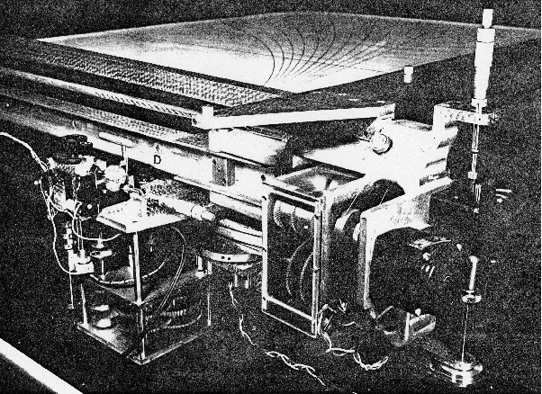
Photo4 Figure 26. Musgrave's migration machine. I don't know about the reader but this looks like a printing press to me.

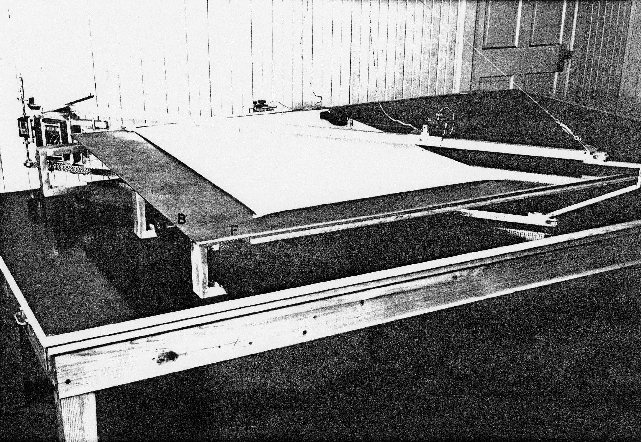
Photo5 Figure 27. Musgrave's version of the design in Figure 20.

In 1959, MIT's WorldWind computer is the first all solid state machine in the world and is quickly followed by scientific offerings from IBM (7090), UNIVAC, Control Data, Texas Instruments (TI) and other computer manufacturers. The TIAC machines from TI are of interest because they were some of the first digital computers to be used in the processing of seismic data. GSI is one of the first seismic contractors to use such machines and continues to use them until the mid 70's (my own experience and that of E. Parma 2004 ()). Initially, programming is difficult, but the stored program nature makes these digital monsters ideal platforms for many of the techniques currently in vogue in seismic imaging. They are in effect general purpose machines that are easily adapted to a variety of purposes. Data must be converted to digital form, but all that's really required is a strong effort in the development of the necessary programs to encapsulate seismic imaging algorithms. As was the case for the original reflection seismograph, there will be tremendous doubts about the new "digital" data and a amazing unwillingness to accept the digital revolution. But, make no mistake, the revolution is on the way. Based on Enders Robinson's 1954 thesis on predictive deconvolution and similar work at the now famous Geophysical Analysis Group (GAG) at MIT, Geophysical Service Incorporated (GSI) (with Backus, Burg, and Schneider) along with Treitel at AMOCO are very likely the first companies to take advantage of these digital initiatives 2004 ().