1936-1953: The age of reflections

What changed all this seems to have happened in the mid 1930's. By now I would presume, several of the larger oil companies including The Texas Company (TEXACO), Amerada Petroleum, the forerunners of EXXON, MOBIL and Chevron, Pan American Petroleum (AMOCO), Standard Oil of New Jersey, Carter Oil, and Continental Oil (CONOCO) were already using or were rapidly adopting the "new" reflection seismic method and doing everything possible to use it commercially. I'm quite sure each such company tended to claim to have been the first to use it and also claim the method as their own. Open discussion of it occurred only if it were absolutely clear that a better proprietary approach was available. In the case of Amerada Petroleum 2004 (), all material, books, manuals, and equipment, related to the seismic method were locked up each night to assure that competitors would not benefit from these proprietary secrets. Since the method was now accepted, it was being used to the fullest extent possible.

As its validity became more and more acceptable and as its usage increased, doubts seem to reenter the picture. Even though this newfangled method appeared to work, there were many places where it produced extremely poor seismic records. These were the so-called no-record areas. Questions arose as to why one could get perfectly acceptable records in one area and none in another. Rieber 1936b () was one of the first to recognize what might be happening.

The appearance of an ideal reflection record is well known to all of those familiar with seismograph work. Definite, well marked bands or patterns of vibrations, more or less parallel to each other are seen to traverse the record. These bands persist in amplitudes sufficient to be readily seen and marked, for a considerable length of record. The good shooting conditions, permitting such records to be taken, occur chiefly in regions where strata are definite and well marked, and relatively flat lying. The appearance of a poor or low grade record is, unfortunately, almost as well known, especially to those who have had occasion to attempt reflection shooting in regions of relatively steep folding or faulting. These poor records, while they contain vibrations of good amplitude persisting for a satisfactory distance down the strip, show very few patterns or line-ups which might be marked as reflections. Furthermore, it is frequently impossible to plot from them any consistent structural condition.

Records of this latter type are customarily marked N. R., presumably meaning no reflections. However, a simple consideration of the space geometry of the reflected wave paths will show that, in very many cases, such confused records are due to the presence of too many, rather than too few, reflected waves. Consider first the fact that such poor records are very frequently obtained in the vicinity of steep folding and faulting, where the rapidly changing attitude of the beds must necessarily result in simultaneous arrival of groups of reflections from a wide variety of different directions.

For example, take the well known case of shooting over a syncline. If we could by some means remove either side of the syncline and shoot for the other side alone, we might expect to get a high grade record showing a succession of relatively parallel bands from which the plotted results would correspond accurately to the dip of the beds in that side of the structure.

Not only does he pinpoint the issues, Rieber goes on to design and construct an analog device for modeling waves from simple but realistic geologically styled models. Figures 8, 9, and 10 are three examples of the models he thought important and the "shadow" images he created. In the first we see what today we would call a diffraction from the end of a truncated bed. The second shows how diffractions define a fault and the third, my favorite, shows us precisely what every interpreter would now recognize as the response of a syncline. To me, these are amazing figures. They clearly represent the use of modeling to provide clues as to why some areas of the Earth produce confused incoherent records. Moreover, they do it at a remarkably early time in the evolution of the seismic method.

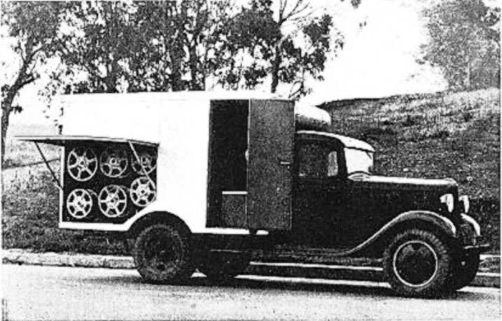
Something even more amazing occurs later in Rieber's paper. Having synthesized the kinds of responses one might expect from more complex subsurface strata, he goes on to try to construct a machine to actually directly estimate apparent dip in a seismic recording. The basic concept was simple and is fully described in Figure 11. From this figure its not surprising that Rieber is one of the first to discuss slant-stacking 1936a () over receiver arrays. In my opinion, the importance of both of Rieber's 1936 papers cannot be overestimated. In the next several years, utilization of emergence angles (Rieber's dip detector) is going to provide the basis for some of the first tiny steps toward fully mechanized seismic imaging. Figure 12 is a picture of Rieber's 1936 instrumentation truck.

Rieber1 Figure 8. Rieber's 1936b () truncated bed shadow graph model with superposed wavefront. The diffraction off the truncated edge is quite clear. This shows an amazing similarity to modern finite difference models

Rieber2 Figure 9. Rieber's 1936b () faulted bed shadow graph model with superposed wavefront. Again the diffraction from the fault is clear.

Rieber3 Figure 10. In this figure Rieber 1936b () shows us the response to a syncline. The top figure is at a shorter time than the bottom. If the reader visualizes when the responses arrive at the surface, the image will be precisely that of a syncline. Compare this to Figure 5

Rieber4 Figure 11. Rieber's 1936b () schematic for detecting arrivals from dipping beds. This is probably the first version of a dip scanning or slant stack device ever devised.

Rieber5 Figure 12. Rieber's 1936 instrumentation truck. The "doghouse" and all.

The bad news of this period of time was war. Undoubtedly World War II put a real crimp in seismic exploration. Seismic surveying certainly did not stop, but the number of scientific minds devoted directly to seismic reflection methods was surely significantly reduced. The focus had to be on the development of the machines of war and the theoretical technology to keep the free world free. This period is probably marked by the likes of the Swedish mathematician Herman Wold, together with Norbert Weiner, C. E. Shannon, and Norman Levinson at MIT. While their pioneering efforts focused mostly on the war effort, they would lead through Shannon's sampling theorem for converting continuous to discrete signals to computational methods for times series analysis, signal processing, and "numerical calculus." This discrete calculus would become better known as Numerical Analysis and form the basis for the finite difference approach to seismic imaging. The foundations for the coming digital revolution were being formed.

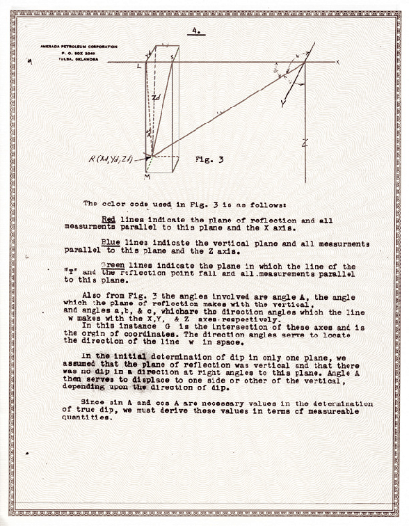
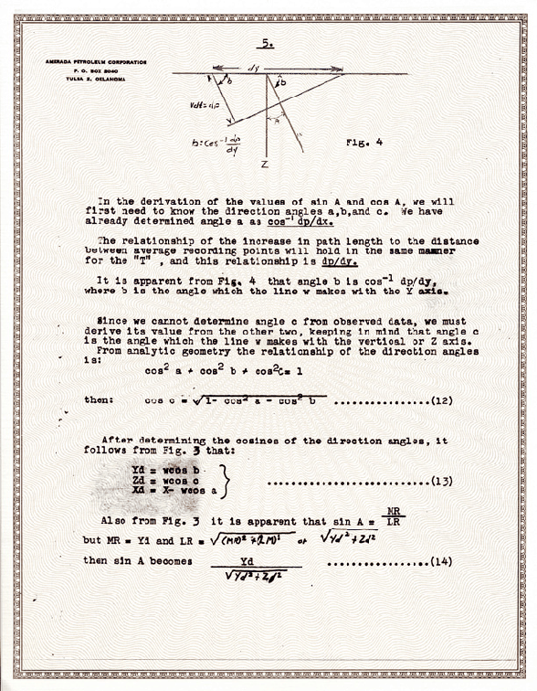
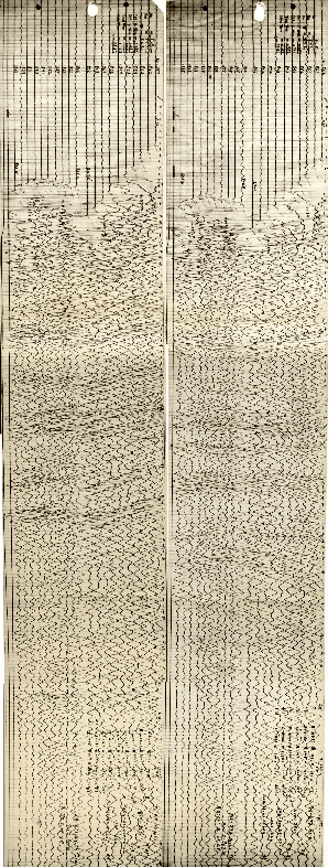
Seismic exploration was still completely in the hands of the doodlebugger. All operations and computations were done in the field, but very likely due to the previously mentioned work of Rieber, and certainly others at the time, the recognition that the world was not really flat began to have an effect. The two pages from a 1940's vintage Amerada Petroleum manual represented in Figures 13, and 14 were part of a five page set that described both the necessary measurements and calculations required to properly position 3D reflections at their correct subsurface location. Although at first glance the formulas here do not appear to have a lot of relevance to seismic imaging, the manner in which this information was used did have a direct relationship. Moreover, they represent a clear recognition that the world was three-dimensional. As a line of seismic data was acquired, the party chief in the field would do the necessary calculations to begin to map a prospective horizon (or maybe horizons). When a significant amount of dip was recognized, a cross spread or "Tee" would be laid out perpendicular to the "straight-two-way" direction of shooting. The next shot would then produce a record similar to one of those in Figure 15. As can be seen, the left-hand side of each record is a normal split-spread response while the right-hand side shows upward sweeping events as a consequence of the perpendicular nature of the receivers in the "Tee" group. There would have been another set of records with the straight-two-way on the right. From picks from this record, the in Figure 13 would be measured. Along with and a suitable set of cosine and sine tables, the true dip vector would be calculated. This vector then defined the new direction of the line. Thus, to the degree possible, lines were shot along the direction of true dip and as a result the map made from the in-field measurements was as close to a 3D migrated map as possible. To my way of thinking this approach is remarkably close to the 3D two-step migration method popularized in the late 1970's and early 1980's.

page4 Figure 13. Page 4 of the Geophysical Research Corporation approach to dip calculations

page5 Figure 14. Page 5 of the Geophysical Research Corporation approach to dip calculations

ComboSmRecords Figure 15. Two late 1940's vintage Amerada Petroleum seismic record showing a "straight-two-way" and a"Tee" record for determining the parameters for the calculations described in Figures - 14. Note that the left hand side is a normal split-spread record while the right-hand side of each record represents the "Tee"

While the pages shown here are from Amerada Petroleum (now Amerada Hess Corporation) and L. Y. Faust 2004 () in the late 1940's, I am quite sure that this kind of process was more or less in vogue at most of the major oil companies and in many research instutitions of this era. C. Hewit Dix's 1952 () and Slotnick's 1959 () books are ample evidence of this. According to Sven Treitel 2004 (), Dix describes and shows a drawing of a "Dip Plotting Machine" or "Dip Swinger" and alludes to a circular slide rule for dip computations described in a 1947 paper by Mansfield.

Many interpreters from this period, some of whom (Hank Adair, Jim Buelow, Richard Brown, Richard Bradley and Octa Otan at Amerada Hess) I had the pleasure of working with, were extremely adept at visually migrating data. They could take one look at an unmigrated section and instantly describe the structure or prospect without even looking at a migrated image of it. This was true even in Gulf of Mexico salt provinces where dips along salt flanks were extreme. I think it would be correct to say that these professionals knew what they were doing and understood it both practically and theoretically. In some sense they were the migration algorithms of their era.

The seismic response from dipping beds is clearly being recognized and understood. It is also clear from what is about to happen that efforts to improve seismic imaging are gathering steam. How, when, and where improvements will come may not always be clear, but what the improvements will be is about to be published and crystallized.